02: An Image is Worth 16x16 Words: Transformers for Image Recognition at Scale(ViT)
在了解了什么是Transformer之后,我们来看看如何将Transformer应用于Computer Vision。Vision Transformer(ViT)是一个将Transformer架构应用于图像分类的模型。它的核心思想是将图像划分为小块(patches),然后将这些小块视为序列数据,类似于处理文本数据。
以下Vision Transformer的主要贡献:
- 首次将 Transformer 成功应用于图像识别任务,表明卷积并不是唯一的选择。
- 证明了大规模预训练(如 JFT-300M)对 ViT 表现至关重要,没有强归纳偏置(inductive bias)时模型更依赖数据。
- 在多个图像分类基准(如 ImageNet)上达到了 SOTA 表现,优于同参数规模的 ResNet。
接下来,我们将详细介绍 Vision Transformer 的架构和实现细节。
1 Vision Transformer Architecture

Vision Transformer 的模型, 如 Figure 1 所示,主要包括以下几个步骤:
- 图像预处理 Section 1.1 :将输入图像划分为固定大小的块(例如 16x16 像素),并将这些块展平和线性嵌入。
- 可学习的位置嵌入 Section 1.2: 为每个图像块添加可学习的位置嵌入,以保留空间信息,并且在开头添加一个分类标记(CLS token)用于最终的分类任务。
- Transformer 编码器 Section 1.3: 使用多层 Transformer 编码器对图像块进行处理,捕捉全局上下文信息。
- 分类头 Section 1.4: 将 Transformer 的输出通过一个简单的全连接层进行分类。
1.1 Patchifying Image
想将Transformer应用图,首先第一个问题就是,如何将图像转换为适合 Transformer 处理的格式?和 Text 数据类型不同,图像数据是二维的,而 Transformer 处理的是一维序列数据。因此,我们需要一种方法将图像转换为一维序列。首先第一个直觉就是,直接将图像展平为一维序列 (Chen et al., n.d.), 如 Figure 2 所示。
然而, 这种方法存在以下显而易见的问题:
- 效率问题:直接展平图像会导致序列长度非常长,计算和存储开销巨大。在 01-Transformer 中,我们提到的随着序列长度的增加,Transformer 的计算复杂度会quadratic 增长,这使得处理高分辨率图像变得不切实际。
…the reliance on low-level pixels as input makes training costly and hinders scaling.
- 缺乏局部信息:直接展平图像会丢失局部结构信息,忽略了图像的二维空间结构(locality、平移不变性),导致模型难以捕捉图像中的空间关系。
既然直接展开不行,那我们可不可以将几个像素组合成一个单元呢?类似于Convolutional Neural Networks(CNN)中的卷积核操作?这就是 Vision Transformer 中的Patchify策略。
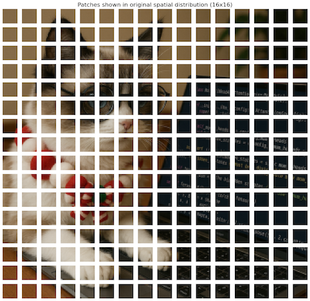
Vision Transformer 采用了Patchify的策略,将图像划分为固定大小的小块(patches),然后将这些小块展平并嵌入到一个一维序列中,如 Figure 3 所示。具体步骤如下:
- 划分图像:将输入图像划分为大小为 \(P \times P\) 的小块(patches),例如 16x16 像素。
- 展平小块:将每个小块展平为一个一维向量。对于每个 \(P \times P\) 的小块,展平后的向量长度为 \(P^2 \times C\),其中 \(C\) 是图像的通道数(例如 RGB 图像的 \(C=3\))。
- 线性嵌入:将展平的小块通过一个线性层(全连接层)嵌入到一个固定的维度 \(D\),通常 \(D\) 是 Transformer 模型的隐藏维度。这样,每个小块就被转换为一个 \(D\) 维的向量。
具体来说,假设输入的图像 \(\mathrm{x} \in \mathbb{R}^{ C \times H \times W }\),经过 Patchify 处理后,得到的图像块为 \(\{ x_i \in \mathbb{R}^{C \times P \times P } \}_{i=1}^N\),其中 \(N = \frac{H \times W}{P^2}\) 是图像块的数量。之前我们将得到的像素块展平为 \(x_i \in \mathbb{R}^{(C \cdot P \cdot P)}\),然后通过线性层 \(W \in \mathbb{R}^{(C \cdot P \cdot P) \times D}\) 嵌入到 \(D\) 维空间,得到 \(\{z_i \in \mathbb{R}^D\}_{i=1}^N\)。
\[ \boxed{ \mathbf{x} \in \mathbb{R}^{C \times H \times W} \quad \xrightarrow{\text{Patchify}} \quad \{ x_i \in \mathbb{R}^{C \times P \times P} \}{i=1}^N \quad \xrightarrow{\text{Flatten}} \quad \{ x_i \in \mathbb{R}^{(C \cdot P \cdot P)} \}_{i=1}^N \quad \xrightarrow{\text{Linear } W \in \mathbb{R}^{(C \cdot P \cdot P) \times D}} \quad \{ z_i \in \mathbb{R}^{D} \}_{i=1}^N } \tag{1}\]
通过这种方式,Vision Transformer 能够将图像转换为适合 Transformer 处理的序列数据,同时保留了局部结构信息。Patchify 的大小 \(P\) 是一个超参数,通常选择为 16 或 32,这取决于输入图像的分辨率和模型的设计。
1.2 Learnable Position Embeddings
解决了如何将图像转换为适合 Transformer 处理的序列数据后,接下来需要考虑的是如何保留图像块之间的位置信息。由于 Transformer 本身不具备处理位置信息的能力,因此需要引入位置嵌入(position embeddings)。 在论文中,使用可学习的位置嵌入:为每个图像块添加一个可学习的位置嵌入向量。
We use standard learnable 1D position embeddings, since we have not observed significant performance gains from using more advanced 2D-aware position embeddings
与Transformer一样,位置的嵌入是一个与输入序列长度相同的向量,每个位置对应一个可学习的参数。具体来说,对于每个图像块 \(z_i\),我们添加一个位置嵌入 \(p_i\),使得最终的输入序列为: \[ \mathbf{z} = \{ z_i + p_i \}_{i=1}^N, \quad \text{where}\ p_i \in \mathbb{R}^D \]
1.2.1 CLS Token
此外,为了进行图像分类,Vision Transformer 在输入序列的开头添加了一个特殊的分类标记(CLS token)(Devlin et al. 2019),这个标记用于最终的分类任务。这个 CLS token 也是一个可学习的向量,通常初始化为零向量。
CLS token 是一个特殊的标记,用于表示整个输入序列的全局信息。在 Vision Transformer 中,CLS token 的位置嵌入也是可学习的。它在 Transformer 编码器处理完所有图像块后,作为分类头 (Section 1.4) 的输入。
1.3 Transformer Encoder
在处理完图像块和位置嵌入后,接下来就是将这些信息输入到 Transformer 编码器中。Vision Transformer 使用了标准的 Transformer 编码器结构,包括多头自注意力机制(Multi-Head Self-Attention)和前馈神经网络(Feed-Forward Neural Network),如 Figure 4 所示.
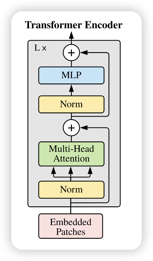
在这里就不再详细介绍 Transformer 编码器的工作原理了,感兴趣的读者可以参考之前的01 Transformer。 不过值得一提的是,normalization的位置,在 Vision Transformer 中,Layer Normalization 被放置在每个子层的输入端(Pre-Norm) ,而不是输出端, 见 Figure 5 。这与原始的 Transformer 设计有所不同.
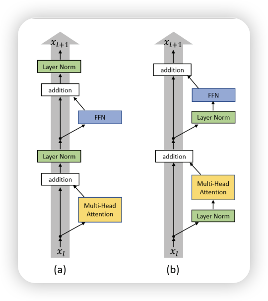
Pre-Norm 的好处是可以更好地稳定训练过程,尤其是在深层网络中。它通过在每个子层之前进行归一化,确保输入的分布在每个子层中保持一致,从而减少梯度消失或爆炸的风险, 并且有助于更好的梯度的传播,并且消除了训练中对warm-up的需求 (Xiong et al. 2020)。
1.4 Classification Head
ViT 的最后一步是分类头,它将 Transformer 编码器的输出用于图像分类任务。具体来说,使用 CLS token 的输出作为图像的全局表示,然后通过一个简单的全连接层进行分类。
\[ \mathbf{y} = \text{softmax}(W_{\text{cls}} \cdot z_{\text{cls}} + b_{\text{cls}}) \tag{2}\]
其中 \(z_{\text{cls}}\) 是 CLS token 的输出,\(W_{\text{cls}} \in \mathbb{R}^{D \times C}\) 和 \(b_{\text{cls}} \in \mathbb{R}^{C}\) 是分类头的权重和偏置。
1.5 ViT Summary
总的来说,再了解了什么是Transformer之后,再了解Vision Transformer就相对简单了。Vision Transformer 的核心思想是将图像划分为小块(patches),然后将这些小块视为序列数据,类似于处理文本数据。通过 Patchify、可学习的位置嵌入、Transformer 编码器和分类头等步骤,ViT 能够有效地处理图像分类任务。 接下来,我们将介绍如何在 PyTorch 中实现 Vision Transformer。
2 PyTorch Implementation
在 PyTorch 中实现 Vision Transformer 的关键步骤包括 Patchify、位置嵌入、Transformer 编码器和分类头。
2.1 Patchify
首先,我们需要实现 Patchify 的操作,将输入图像划分为小块并展平。可以使用一个卷积层来实现这一点,如 Section 1.1 中所述。
class PatchEmbedding(nn.Module):
    def __init__(self, config: ModelConfig):
        super().__init__()

        self.conv = nn.Conv2d(
            in_channels=config.num_channels,
            out_channels=config.hidden_dim,
            kernel_size=config.patch_size,
            stride=config.patch_size,
            padding="valid" if config.patch_size == 16 else "same",
        )

    def forward(self, imgs: torch.Tensor) -> torch.Tensor:
        """
        imgs: (batch_size, num_channels, height, width)
        Returns: (batch_size,  num_patches_height, num_patches_width, hidden_dim)
        """
        # (B, C, H, W) -> (B, hidden_dim, H', W')
        x = self.conv(imgs)

        # (B, hidden_dim, H', W') -> (B, hidden_dim, H' * W')
        x = x.flatten(2)

        # (B, hidden_dim, H' * W') -> (B, H' * W', hidden_dim)
        x = x.transpose(1, 2)
        return x
2.2 Learnable Position Embeddings
接下来,我们需要实现可学习的位置嵌入。可以直接设置可学习的参数,并在前向传播中添加到图像块的嵌入上。主要注意的是,除了patches的嵌入外,我们还需要添加一个可学习的 CLS token,所有总共是 \((H \cdot W / P^2 + 1)\) 个位置嵌入。
class PositionalEncoding(nn.Module):
    def __init__(self, config: ModelConfig):
        super().__init__()

        self.positional_embedding = nn.Parameter(
            torch.randn(
                1,
                (config.image_size // config.patch_size) ** 2 + 1,
                config.hidden_dim,
            )
        )

        self.cls_token = nn.Parameter(torch.randn(1, 1, config.hidden_dim))

    def forward(self, x: torch.Tensor):
        """
        x: (batch_size, num_patches, hidden_dim)
        Returns: (batch_size, num_patches, hidden_dim)
        """
        # Add positional encoding to the input tensor
        batch_size = x.size(0)

        pos_embedding = self.positional_embedding.expand(batch_size, -1, -1)
        cls_token = self.cls_token.expand(batch_size, -1, -1)

        x = torch.cat((cls_token, x), dim=1)
        return x + pos_embedding
在这里,我们添加了一个可学习的 CLS token,并将其与图像块的嵌入拼接在一起。
2.3 Transformer Encoder
接下来是Transformer 编码器的实现。分成 Attention和 FeedForward 两个部分。注意这里的 Layer Normalization 是 Pre-Norm 的形式。想较于原始的Encoder,ViT的实现,比较简单,我们不需要实现 Masked Attention,因为 Vision Transformer 只处理图像块的全局上下文。 #### Multi-Head Attention
def scale_dot_product(query, key, value):
    """
    Scaled Dot-Product Attention
    Args:
        query: Tensor of shape (batch_size, num_heads, seq_length, d_k)
        key: Tensor of shape (batch_size, num_heads, seq_length, d_k)
        value: Tensor of shape (batch_size, num_heads, seq_length, d_v)
    Returns:
        output: Tensor of shape (batch_size, num_heads, seq_length, d_v)
    """

    d_k = query.size(-1)
    scores = torch.matmul(query, key.transpose(-2, -1)) / math.sqrt(d_k)
    attn = F.softmax(scores, dim=-1)
    output = torch.matmul(attn, value)
    return output

class MHA(nn.Module):
    def __init__(self, config: ModelConfig):
        super().__init__()

        self.num_heads = config.num_heads
        self.hidden_dim = config.hidden_dim
        self.head_dim = config.hidden_dim // config.num_heads

        self.query_proj = nn.Linear(config.hidden_dim, config.hidden_dim)
        self.key_proj = nn.Linear(config.hidden_dim, config.hidden_dim)
        self.value_proj = nn.Linear(config.hidden_dim, config.hidden_dim)
        self.out_proj = nn.Linear(config.hidden_dim, config.hidden_dim)

        self.dropout = nn.Dropout(config.attention_dropout_rate)

    def forward(self, x: torch.Tensor):
        """
        x: (batch_size, num_patches, hidden_dim)
        Returns: (batch_size, num_patches, hidden_dim)
        """
        batch_size = x.size(0)

        # Project inputs to query, key, value
        query = (
            self.query_proj(x)
            .view(batch_size, -1, self.num_heads, self.head_dim)
            .transpose(1, 2)
        )
        key = (
            self.key_proj(x)
            .view(batch_size, -1, self.num_heads, self.head_dim)
            .transpose(1, 2)
        )
        value = (
            self.value_proj(x)
            .view(batch_size, -1, self.num_heads, self.head_dim)
            .transpose(1, 2)
        )

        # Apply scaled dot-product attention
        attn_output = scale_dot_product(query, key, value)

        # Concatenate heads and project back to hidden dimension
        attn_output = (
            attn_output.transpose(1, 2)
            .contiguous()
            .view(batch_size, -1, self.hidden_dim)
        )
        output = self.out_proj(attn_output)

        output = self.dropout(output)

        return output
2.3.1 Feed-Forward Network
class FFN(nn.Module):
    def __init__(self, config: ModelConfig):
        super().__init__()
        self.fc1 = nn.Linear(config.hidden_dim, config.mlp_dim)
        self.fc2 = nn.Linear(config.mlp_dim, config.hidden_dim)
        self.dropout = nn.Dropout(config.dropout_rate)

    def forward(self, x: torch.Tensor):
        """
        x: (batch_size, num_patches, hidden_dim)
        Returns: (batch_size, num_patches, hidden_dim)
        """
        x = F.relu(self.fc1(x))
        x = self.dropout(x)
        x = self.fc2(x)
        return x
2.3.2 Pre-Normalization
在 Vision Transformer 中,Layer Normalization 被放置在每个子层的输入端(Pre-Norm) ,而不是输出端, 见 Figure 5 。
class EncoderBlock(nn.Module):
    def __init__(self, config: ModelConfig):
        super().__init__()
        self.mha = MHA(config)
        self.ffn = FFN(config)
        self.norm1 = LayerNorm(config.hidden_dim)
        self.norm2 = LayerNorm(config.hidden_dim)

    def forward(self, x: torch.Tensor):
        """
        x: (batch_size, num_patches, hidden_dim)
        Returns: (batch_size, num_patches, hidden_dim)
        """
        # Multi-head attention
        redisual = x
        x = self.norm1(x)
        x = redisual + self.mha(x)

        # Feed-forward network
        redisual = x
        x = self.norm2(x)
        x = x + self.ffn(x)

        return x
2.4 Classification Head
之后是分类头的实现。我们使用 CLS token 的输出作为图像的全局表示,然后通过一个简单的全连接层进行分类。
class MLPHead(nn.Module):
    def __init__(self, config: ModelConfig):
        super().__init__()
        self.fc1 = nn.Linear(config.hidden_dim, config.mlp_dim)
        self.fc2 = nn.Linear(config.mlp_dim, config.num_classes)
        self.dropout = nn.Dropout(config.dropout_rate)

    def forward(self, x: torch.Tensor):
        """
        x: (batch_size, num_patches, hidden_dim)
        Returns: (batch_size, num_classes)
        """
        # Use the CLS token for classification
        cls_token = x[:, 0, :]
        x = F.relu(self.fc1(cls_token))
        x = self.dropout(x)
        x = self.fc2(x)

        return x
2.5 ViT Model
最后,我们将所有组件组合在一起,形成完整的 Vision Transformer 模型。
class ViT(nn.Module):
    def __init__(self, config: ModelConfig):
        super().__init__()
        self.patch_embedding = PatchEmbedding(config)
        self.positional_encoding = PositionalEncoding(config)
        self.encoder = Backbone(config)
        self.mlp_head = MLPHead(config)

    def forward(self, imgs: torch.Tensor) -> torch.Tensor:
        """
        imgs: (batch_size, num_channels, height, width)
        Returns: (batch_size, num_classes)
        """
        x = self.patch_embedding(imgs)
        x = self.positional_encoding(x)
        x = self.encoder(x)
        x = self.mlp_head(x)

        return x
2.6 训练集
在这个演示中,我们将使用Intel Image Classification 数据集进行训练。