LLM Part1: Architecture
This is the part 1 of the LLM series, architecture. In this blog, we will going through different transformer architectures that power LLMs. Such as position encoding, attention mechanisms, and more. In the end, we will explore some SOTA LLM architectures, and study how to they combine those techniques to achieve better performance. We are going from bottom to up:
- Position Encoding
- Attention Mechanism
- Feed Forward Network & Mixture of Experts
- Output Layer
Besides that, we will also explore different normalization techniques, such as Layer Normalization and RMS Normalization, and the different position of the normalization layers within the architecture. Then, we will going through the training process and how to effectively train these architectures.
1 The overview of transformer model
The Transformer model, originally proposed in the paper “Attention is All You Need” (Vaswani et al. 2023), is a neural network architecture designed to process sequential data, such as natural language. With the high parallelization capabilities of transformers, they have become the foundation for many state-of-the-art natural language processing models. Nowadays, the most LLM are based on the variance of the transformer architecture. The transformer architecture consists of an encoder and a decoder, each composed of multiple layers of self-attention and feed-forward networks, as displayed in the Figure 1.
For those who are not familiar with the transformer architecture, it is important to understand its key components and how they work together to process sequential data. I highly recommend this post: 01-Attention is All You Need, which I implement the transformer from scratch, not just transformer model, but also Adam optimizer, label smoothing, and training loop of the transformer.
2 Position Encoding
Since the transformer architecture does not have any recurrence or convolution, it is necessary to provide some information about the position of the tokens in the sequence. This is achieved through position encoding, which adds a unique positional vector to each token embedding. There are several methods for implementing position encoding, including:
- Absolute Position Encoding: This method assigns a unique position embedding to each position in the input sequence, regardless of the content of the tokens. This can be useful for tasks where the absolute position of tokens is important. One common approach is to use a fixed sinusoidal function to generate the position embeddings.
- Learned Position Encoding: In this approach, the model learns a set of position embeddings during training, similar to word embeddings. This allows the model to adapt the position encodings to the specific task and dataset.
- Relative Position Encoding: This method encodes the relative distances between tokens, rather than their absolute positions. This can be particularly useful for tasks where the relationships between tokens are more important than their specific locations in the sequence.
First, let’s dive into the absolute position encoding.
2.1 Learned Position Encoding
In the absolute position encoding, we put our position information into fixed sinusoidal functions. It is hand-crafted for specific tasks and does not adapt to the data. So, is it possible to learn position encodings from the data itself? It is possible, and this leads us to the concept of learned position encodings. The learned position encodings are typically implemented as additional trainable parameters in the model. Instead of using fixed sinusoidal functions, the model learns to generate position embeddings that are optimized for the specific task and dataset.
This method is used in such as Vision Transformers (Dosovitskiy et al. 2021).
2.2 Absolute Position Encoding
As used in the (Vaswani et al. 2023), absolute position encoding assigns a unique position embedding to each position in the input sequence, regardless of the content of the tokens. One common approach is to use a fixed sinusoidal function to generate the position embeddings. For example: for each position \(pos\), the position embedding \(PE(pos)\) can be defined as:
\[ \begin{aligned} \text{PE}(pos, 2i) &= \sin\!\left(pos \times \frac{1}{10,000^{2i/d_{\text{model}}}}\right) \\ \text{PE}(pos, 2i+1) &= \cos\!\left(pos \times \frac{1}{10,000^{2i/d_{\text{model}}}}\right) \end{aligned} \tag{1}\]
where
- \(d_{\text{model}}\) is the dimensionality of the embeddings.
- \(i\) is the index of the embedding dimension. The sin function is applied to the even indices \(2i\), while the cos function is applied to the odd indices \(2i+1\).
We can illustrate the encoding as following:

There are several properties can be read from the Figure 2 and Equation 1:
Periodicity: The sine and cosine functions used in the position encoding have a periodic nature, which allows the model to easily learn to attend to relative positions. This is evident in Figure 2 (a), where the position encodings exhibit similar patterns for different sequence lengths.
Dimensionality: The choice of \(d_{\text{model}}\) affects the granularity of the position encodings. As shown in Figure 2 (b), increasing the dimensionality results in more fine-grained position encodings, which can help the model capture more subtle positional information.
The low-dimension part of the dmodel is change more frequently than the high-dimension part, allowing the model to adapt more easily to different input lengths.
We chose this function because we hypothesized it would allow the model to easily learn to attend by relative positions, since for any fixed offset \(k\), \(PE_{pos+k}\) can be represented as a linear function of \(PE_{pos}\). Attention Is All You Need
How to understand this sentence. Let’s first redefine the position encoding. \[ \begin{aligned} \mathrm{PE}(pos,2i) &= \sin\!\Big(\tfrac{pos}{\alpha_i}\Big), \\ \mathrm{PE}(pos,2i+1) &= \cos\!\Big(\tfrac{pos}{\alpha_i}\Big). \end{aligned} \] where \(\alpha_i = 10,000^{2i/d_{\text{model}}}\). And we consider \((2i, 2i+1)\) as one pair. Now, consider the same pair at position \(pos + k\). We can write the position encoding as:
\[ \begin{align} \mathrm{PE}(pos+k,2i) &= \sin\!\Big(\tfrac{pos+k}{\alpha_i}\Big) = \sin\!\Big(\tfrac{pos}{\alpha_i}\Big)\cos\!\Big(\tfrac{k}{\alpha_i}\Big) + \cos\!\Big(\tfrac{pos}{\alpha_i}\Big)\sin\!\Big(\tfrac{k}{\alpha_i}\Big) \\ \mathrm{PE}(pos+k,2i+1) &= \cos\!\Big(\tfrac{pos+k}{\alpha_i}\Big) =\cos\!\Big(\tfrac{pos}{\alpha_i}\Big)\cos\!\Big(\tfrac{k}{\alpha_i}\Big) - \sin\!\Big(\tfrac{pos}{\alpha_i}\Big)\sin\!\Big(\tfrac{k}{\alpha_i}\Big) \end{align} \tag{2}\]
Angle addition formulas: \[ \begin{align*} &\sin(a+b) = \sin(a)\cos(b) + \cos(a)\sin(b) \\ &\cos(a+b) = \cos(a)\cos(b) - \sin(a)\sin(b) \end{align*} \]
Write this as vector form:
\[ \mathbf{p}_{pos}^{(i)} = \begin{bmatrix} \sin(pos/\alpha_i) \\ \cos(pos/\alpha_i) \end{bmatrix} \]
Then \(\mathbf{p}_{pos+k}^{(i)}\) equal to: \[ \mathbf{p}_{pos+k}^{(i)} = \underbrace{ \begin{bmatrix} \cos(\tfrac{k}{\alpha_i}) & \ \ \sin(\tfrac{k}{\alpha_i}) \\ -\sin(\tfrac{k}{\alpha_i}) & \ \ \cos(\tfrac{k}{\alpha_i}) \end{bmatrix} }_{\displaystyle R_i(k)} \ \mathbf{p}_{pos}^{(i)} \]
Notice that \(R_i(k)\) is known as rotation matrix which only depends on the relative position \(k\) and not on the absolute position \(pos\). This is the key insight that allows the model to generalize to different positions.
Stacking all pairs, \[ \mathrm{PE}(pos+k) = \underbrace{ \begin{pmatrix} \cos\!\big(\tfrac{k}{\alpha_1}\big) & \sin\!\big(\tfrac{k}{\alpha_1}\big) & 0 & 0 & \cdots & 0 & 0 \\ -\sin\!\big(\tfrac{k}{\alpha_1}\big) & \ \cos\!\big(\tfrac{k}{\alpha_1}\big) & 0 & 0 & \cdots & 0 & 0 \\ 0 & 0 & \cos\!\big(\tfrac{k}{\alpha_2}\big) &\sin\!\big(\tfrac{k}{\alpha_2}\big) & \cdots & 0 & 0 \\ 0 & 0 & -\sin\!\big(\tfrac{k}{\alpha_2}\big) & \ \cos\!\big(\tfrac{k}{\alpha_2}\big) & \cdots & 0 & 0 \\ \vdots & \vdots & \vdots & \vdots & \ddots & \vdots & \vdots \\ 0 & 0 & 0 & 0 & \cdots & \cos\!\big(\tfrac{k}{\alpha_{d/2}}\big) & \sin\!\big(\tfrac{k}{\alpha_{d/2}}\big) \\ 0 & 0 & 0 & 0 & \cdots & -\sin\!\big(\tfrac{k}{\alpha_{d/2}}\big) & \ \cos\!\big(\tfrac{k}{\alpha_{d/2}}\big) \end{pmatrix} }_{R(k)} \cdot \underbrace{ \begin{pmatrix} \sin(\tfrac{k}{\alpha_1}) \\ \cos(\tfrac{k}{\alpha_1}) \\ \sin(\tfrac{k}{\alpha_2}) \\ \cos(\tfrac{k}{\alpha_2}) \\ \vdots \\ \sin(\tfrac{k}{\alpha_{d/2}}) \\ \cos(\tfrac{k}{\alpha_{d/2}}) \end{pmatrix} }_{\mathrm{PE}(pos)} \]
where \(R(k)\) is block-diagonal with those \(2\times2\) rotations, \(R(k)\) depends on \(k\) but not on \(pos\) → a linear map of \(\mathrm{PE}(pos)\).
2.3 Relative Position Encoding
Relative Position Encoding, first proposed in Transformer-XL (Dai et al. 2019), then adaptive in different language model.
\[ A_{i,j} = \underbrace{Q_i^\top K_j}_{\text{content-based addressing}} + \underbrace{Q_i^\top R_{i-j}}_{\text{content-dependent positional bias}} + \underbrace{u^\top K_j}_{\text{global content bias}} + \underbrace{v^\top R_{i-j}}_{\text{global positional bias}} \]
where:
- \(Q_i \in \mathbb{R}^d\): query vector at position \(i\)
- \(K_j \in \mathbb{R}^d\): key vector at position \(j\)
- \(R_{i-j} \in \mathbb{R}^d\): embedding of the relative distance \((i-j)\)
- \(u, v \in \mathbb{R}^d\): learnable global bias vectors
- \(A_{i,j}\): unnormalized attention score between position \(i\) and \(j\)
import torch
import torch.nn as nn
import torch.nn.functional as F

class RelPositionalEncoding(nn.Module):
    def __init__(self, d_model, max_len=5000):
        super().__init__()
        self.d_model = d_model

        # relative positions: range [-max_len, max_len]
        range_len = max_len * 2 + 1
        self.rel_emb = nn.Embedding(range_len, d_model)

        # trainable biases u, v (Transformer-XL)
        self.u = nn.Parameter(torch.Tensor(d_model))
        self.v = nn.Parameter(torch.Tensor(d_model))

    def forward(self, q, k, seq_len):
        B, H, L, Dh = q.size()

        # (L, L): relative position indices
        pos_idx = torch.arange(L, dtype=torch.long, device=q.device)
        rel_idx = pos_idx[None, :] - pos_idx[:, None]  # i-j
        rel_idx = rel_idx + seq_len  # shift to [0, 2*max_len]
        rel_pos_emb = self.rel_emb(rel_idx)  # (L, L, d_model)

        # compute QK^T (content-based)
        content_score = torch.matmul(q, k.transpose(-2, -1))  # (B, H, L, L)

        # project queries with R
        rel_q = q + self.v.view(1, 1, 1, -1)  # add bias v
        rel_score = torch.einsum('bhld,lrd->bhlr', rel_q, rel_pos_emb)

        # add global content bias (u)
        content_bias = torch.einsum('d,bhjd->bhj', self.u, k).unsqueeze(2)

        # total score
        logits = content_score + rel_score + content_bias
        return logits / (Dh ** 0.5)  # scale as in attention
2.4 RoPE (Rotary Position Embedding)
So far we have see the absolute position encoding and relative position encoding. However, there is an problem with absolute position encoding. For example, for two sentence:
- Every Day I will go to gym
- I will go to gym every day
The absolute position encoding is totally different from two sentences, even though they have the same words and means. On the other hand, the problem of the relative position encoding is that it does not capture the absolute position information, which is crucial for understanding the meaning of the sentences for some task such as text summarization.
RoPE (Su et al. 2023) is a method combine those two. The vector rotated certain degree according to the absolute position in the sentence. On the other hand, it relative position information is preserved. According to Equation 2, the relative position is not related to the position.
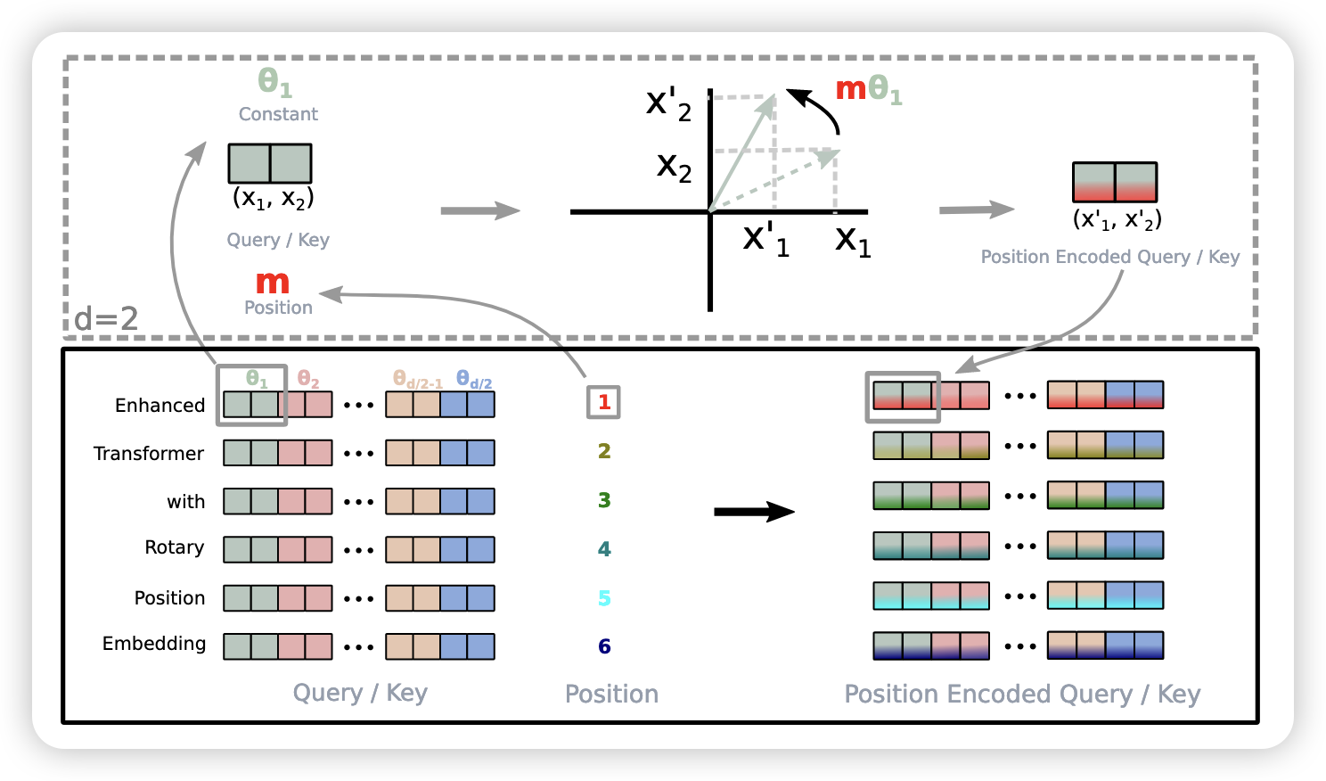
\[ R_{\Theta,m}^{d} \mathbf{x} = \begin{pmatrix} x_1\\ x_2\\ x_3\\ x_4\\ \vdots\\ x_{d-1}\\ x_d \end{pmatrix} \otimes \begin{pmatrix} \cos(m\theta_{1})\\ \cos(m\theta_{1})\\ \cos(m\theta_{2})\\ \cos(m\theta_{2})\\ \vdots\\ \cos\!\big(m\theta_{d/2}\big)\\ \cos\!\big(m\theta_{d/2}\big) \end{pmatrix} + \begin{pmatrix} - x_2\\ x_1\\ - x_4\\ x_3\\ \vdots\\ - x_d\\ x_{d-1} \end{pmatrix} \otimes \begin{pmatrix} \sin(m\theta_{1})\\ \sin(m\theta_{1})\\ \sin(m\theta_{2})\\ \sin(m\theta_{2})\\ \vdots\\ \sin\!\big(m\theta_{d/2}\big)\\ \sin\!\big(m\theta_{d/2}\big) \end{pmatrix} \tag{3}\]
where
\[ \theta_{i,d} = \frac{1}{10,000^{2(i - 1) / d}} ,\quad i \in [1, 2, \dots, d / 2 ] \]
As we can see, to implement the RoPE in code, we can:
- Construct
cosandsinmatrices for the given input dimensions and maximum position. - Apply the rotation to the input embeddings using the constructed matrices.
One thing always bother me about this implementation is that the rotate_half function actually swap pair of the last dimension as mentioned in the paper. For example:
>>> x = torch.arange(0, 24).reshape(3, 8) # (B, D)
>>> x
tensor([[ 0,  1,  2,  3,  4,  5,  6,  7],
        [ 8,  9, 10, 11, 12, 13, 14, 15],
        [16, 17, 18, 19, 20, 21, 22, 23]])
>>> x1 = rotate_half(x)
>>> x1
tensor([[ -4,  -5,  -6,  -7,   0,   1,   2,   3],
        [-12, -13, -14, -15,   8,   9,  10,  11],
        [-20, -21, -22, -23,  16,  17,  18,  19]])
The above function just change the x to [-x_{d//2}, ..., -x_{d}, x_0, ..., x_{d//2-1}]
Check this linkif you are interested.
If this really bother you, you can just implement like this:
def rotate_half_v2(x):
    # Assume x is (B, D)
    x = x.reshape(x.shape[0], -1, 2)
    x1, x2 = x.unbind(dim = -1)
    x = torch.stack((-x2, x1), dim = -1)
    return x.reshape(x.shape[0], -1)
which is same as they mentioned in the paper.
>>> x
tensor([[ 0,  1,  2,  3,  4,  5,  6,  7],
        [ 8,  9, 10, 11, 12, 13, 14, 15],
        [16, 17, 18, 19, 20, 21, 22, 23]])
>>> x2 = rotate_half_v2(x)
>>> x2
tensor([[ -1,   0,  -3,   2,  -5,   4,  -7,   6],
        [ -9,   8, -11,  10, -13,  12, -15,  14],
        [-17,  16, -19,  18, -21,  20, -23,  22]])
Or
def rotate_half_v3(x: torch.Tensor) -> torch.Tensor:
    y = torch.empty_like(x)
    y[..., ::2] = -x[..., 1::2]  # even positions get -odd
    y[..., 1::2] =  x[..., ::2]  # odd positions get even
    return y

>>> x3 = rotate_half_v3(x)
>>> x3
tensor([[ -1,   0,  -3,   2,  -5,   4,  -7,   6],
        [ -9,   8, -11,  10, -13,  12, -15,  14],
        [-17,  16, -19,  18, -21,  20, -23,  22]])
The other implementation of the RoPE is reply on the complex number. We can treat 2D vector \((x, y)\) as a complex number \(z = x + iy\), and the rotation can be done by multiplying with a complex exponential:
\[ z' = z \cdot e^{i\theta} = (x + iy) \cdot (\cos \theta + i \sin \theta) = (x \cos \theta - y \sin \theta) + i (x \sin \theta + y \cos \theta) \]
Code adapted from LLaMA model
2.5 ALIBI
(Press, Smith, and Lewis 2022)
AliBi: simple, monotonic bias → strong extrapolation, lower overhead.
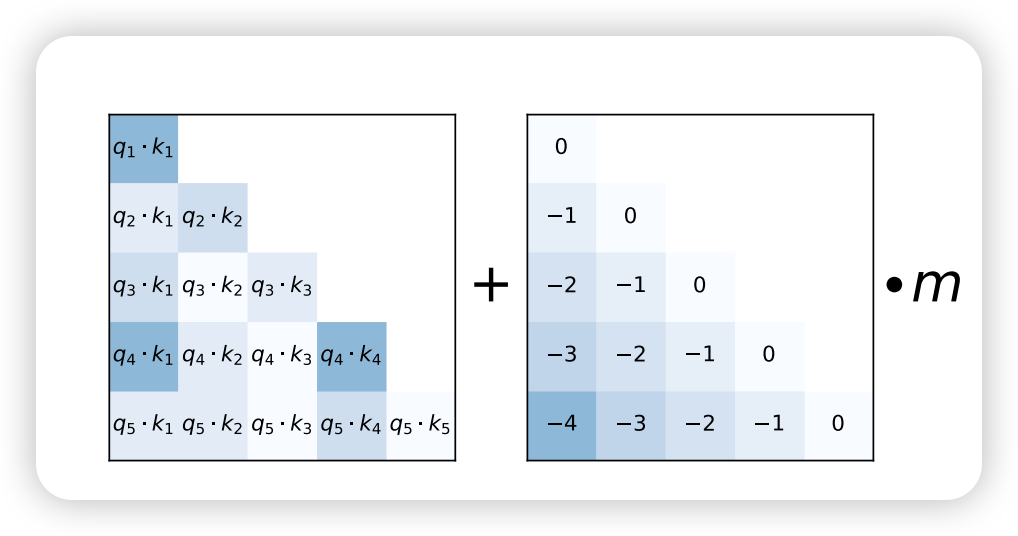
So far, for the position embedding, we modify the Q, K to add the position information for attention to calculate. However, is it possible to directly modify the attention score? To notify them the position information? This is exactly what ALIBI does. The ALIBI (Attention with Linear Biases) method introduces a linear bias to the attention scores based on the distance between tokens. The bias is added directly to the attention score before applying the softmax function. Mathematically:
\[ \operatorname{softmax}\!\Big( q_i k_j^\top \;+\; m \cdot (-(i-j)) \Big) \]
where:
- \(q_i \in \mathbb{R}^d\): query vector at position \(i\)
- \(k_j \in \mathbb{R}^d\): key vector at position \(j\)
- \(m \in \mathbb{R}\): slop (head-dependent constant)
- \((i - j) \geq 0\): relative distance
For example, for query \(i\), the logits against all keys \([0, 1, \dots, i ]\) become: \[ \ell_i \;=\; \Big[\, q_i k_0^\top - m(i-0),\; q_i k_1^\top - m(i-1),\; \ldots,\; q_i k_{i-1}^\top - m(1),\; q_i k_i^\top \,\Big] \]
2.6 Extend to longer context
So far, for all the position encoding we discussed, it has one main drawback: it fixed maximum context length during training.
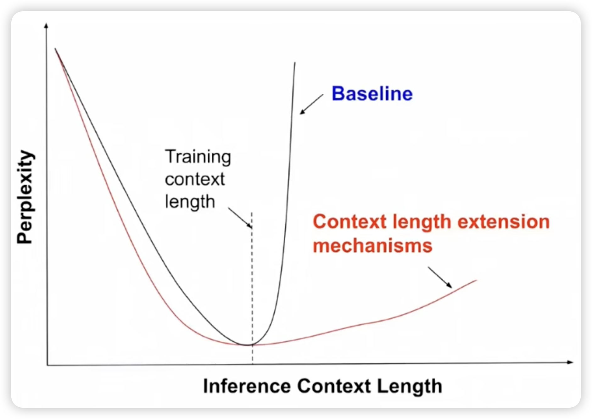
When we are training on the fixed context length, the model learns to attend to the positions within that context. However, during inference, we may want to extend the context length beyond what the model was trained on. This is where the challenge lies. One way is to train a longer context length model from the beginning. However this requires more computational resources and may not be feasible for all applications. So, we need to find a way to adapt the model to longer contexts without retraining it from scratch.
There are several approaches to address this issue. Let’s discuss a few of them.
2.6.1 Linear Position Interpolation
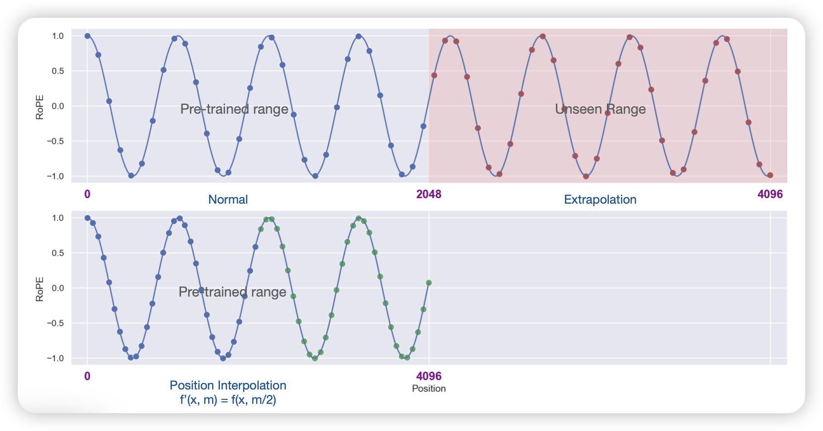
decreases the frequencies of the basis functions so that more tokens fit within each period. The position interpolation (Chen et al. 2023) mentioned that we can just linearly interpolate the position embeddings for the extended context. This allows the model to generate position embeddings for longer sequences without requiring additional training. It just rescale the \(m\) base in the RoPE by: \[ f'(\mathbf{x}, m) = f(\mathbf{x}, m\frac{L}{L'}) \] where \(L\) is the original context length and \(L'\) is the new context length.
2.6.2 NTK-Aware Position Interpolation
The Linear Position Interpolation, if it was possible to pick the correct scale parameter dynamically based on the sequence length rather than having to settle for the fixed tradeoff of maximum sequence length vs. performance on shorter sequences. The NTK-Aware Position Interpolation method leverages the Neural Tangent Kernel (NTK) framework to adaptively adjust the position embeddings during inference. By analyzing the model’s behavior in the NTK regime, we can identify the optimal scaling factors for different sequence lengths, allowing for more effective extrapolation of position information.
\[ \alpha^{\text{NTK-RoPE}}_{j} = \kappa^{-\frac{2j}{d_k}} \]
2.6.3 YaRN
another RoPE extension method, uses “NTK-by-parts” interpolation strategies across different dimensions of the embedding space and introduces a temperature factor to adjust the attention distribution for long inputs. But RoPE cannot extrapolate well to sequences longer than training (e.g., a model trained on 2K tokens struggles at 8K).
\[ \alpha^{\mathrm{YaRN}}_{j} = \frac{(1-\gamma_j)\,\tfrac{1}{t} + \gamma_j}{\sqrt{T}} \,. \]
YaRN modifies RoPE to support longer context windows while preserving model stability. (Peng et al. 2023)
3 Normalization
3.1 Layer Normalization vs. RMS Normalization
The Layer Normalization (Ba, Kiros, and Hinton 2016) is a technique to normalize the inputs across the features for each training example. It is defined as:
\[ \text{LayerNorm}(x) = \frac{x - \mu}{\sigma + \epsilon} \cdot \gamma + \beta \tag{4}\] where:
- \(\mu(x)\): the mean of the input features.
- \(\sigma(x)\): the standard deviation of the input features.
- \(\gamma\): a learnable scale parameter.
- \(\beta\): a learnable shift parameter.
There are two learnable parameters in Layer Normalization: \(\gamma\) and \(\beta\), which have the same shape as the input features \(d_{\text{model}}\).
However, in the Root Mean Square(RMS) Normalization, proposed in (Zhang and Sennrich 2019), that we remove the mean from the normalization process. The RMS Normalization is defined as:
\[ \text{RMSNorm}(x) = \frac{x}{\sqrt{\frac{1}{d} \sum_{i=1}^{d} x_i^2 + \epsilon}} \cdot \gamma \tag{5}\] where:
- \(\epsilon\): a small constant to prevent division by zero.
- \(\gamma\): a learnable scale parameter, which has the same shape as the input features \(d_{\text{model}}\).
As we can see, the main difference between Layer Normalization and RMS Normalization is the removal of the mean from the normalization process, and remove the learnable shift parameter \(\beta\). There are several advantage of that:
- Simplicity: RMS Normalization is simpler and requires fewer parameters, making it easier to implement and faster to compute. For model with \(d_{\text{model}} = 512\), 8 layers, each layer has 2 normalization. Than the reduction number of parameter is up to \(512 \times 8 \times 2 = 8192\) parameters.
- Fewer operations: no mean subtraction, no bias addition.
- Saves memory bandwidth, which is often the bottleneck in GPUs (not FLOPs).
- While reduce the number of parameters, it also maintains similar performance.
3.2 Pre-Layer Normalization vs. Post-Layer Normalization
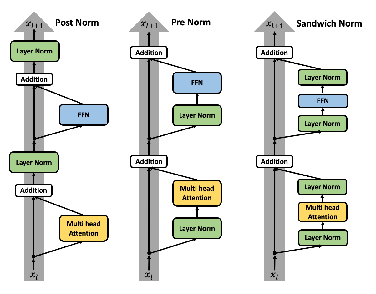
One main good reason why Pre-Layer Normalization is perform bettern than the Post-Layer Normalization is that, according to (Xiong et al. 2020), the help the gradient flow back through the network without disrupting the residual connections. When using the Pre-Layer Normalization, it tends to converge faster and more stably. And the initlization methods is become less sensitive to the scale of the inputs.
There are third type of the normalization position by (Ding et al. 2021) called sandwiched normalization, which is a combination of pre-layer and post-layer normalization. Is is proposed to improve the training for the text-image pair.
One generalizable lesson is that we should keep residual connections “clean” identity paths.
3.3 QK Norm
There is another normalization method called Query-Key Normalization (QK Norm), which is designed to improve the attention mechanism by normalizing the query and key vectors before computing the attention scores.
4 Attention Mechanism
Now, we have arrive the most important component of the transformer architecture: the attention mechanism. There are many efforts and research directions aimed at improving the attention mechanism. we first discuss the standard multi-headed attention, proposed in (Vaswani et al. 2023). And than analysis the time complexity of the the algorithm. Layer see different improvements through change algorithm or better utilize the hardware.
4.1 Multi Headed Attention
The standard multi headed attention is defined as:
\[ \text{MultiHead}(Q, K, V) = \text{Concat}(\text{head}_1, \ldots, \text{head}_h)W^O \tag{6}\]
where each head is computed as:
\[ \text{head}_i = \text{Attention}(QW_i^Q, KW_i^K, VW_i^V) \tag{7}\] with \(W_i^Q\), \(W_i^K\), and \(W_i^V\) being learned projection matrices.
And the attention function, usually is scaled dot-product attention, is defined as: \[ \text{Attention}(Q, K, V) = \text{softmax}\left(\frac{QK^T}{\sqrt{d_k}}\right)V \tag{8}\]
where \(d_k\) is the dimension of the keys. The reason for the scaling factor \(\sqrt{d_k}\) is to counteract the effect of large dot-product values by the large dimension of \(K\), which can push the softmax function into regions with very small gradients.
4.1.1 Time Complexity of Scaled Dot-Product Attention
The time complexity of the scaled dot-product attention mechanism can be analyzed as follows:
- Query-Key Dot Product: The computation of the dot product between the query and key matrices has a time complexity of \(O(n^2 d_k)\), where \(n\) is the sequence length and \(d_k\) is the dimension of the keys.
- Softmax Computation: The softmax function is applied to the dot product results, which has a time complexity of \(O(n^2)\).
- Value Weighting: The final step involves multiplying the softmax output with the value matrix, which has a time complexity of \(O(n^2 d_v)\), where \(d_v\) is the dimension of the values.
Overall, the time complexity of the scaled dot-product attention is dominated by the query-key dot product and can be expressed as:
\[ O(n^2 (d_k + d_v)) \tag{9}\]
As we can see, the time complexity is quadratic in the sequence length, which can be a bottleneck for long sequences / contexts. Let’s see how we can improve it.
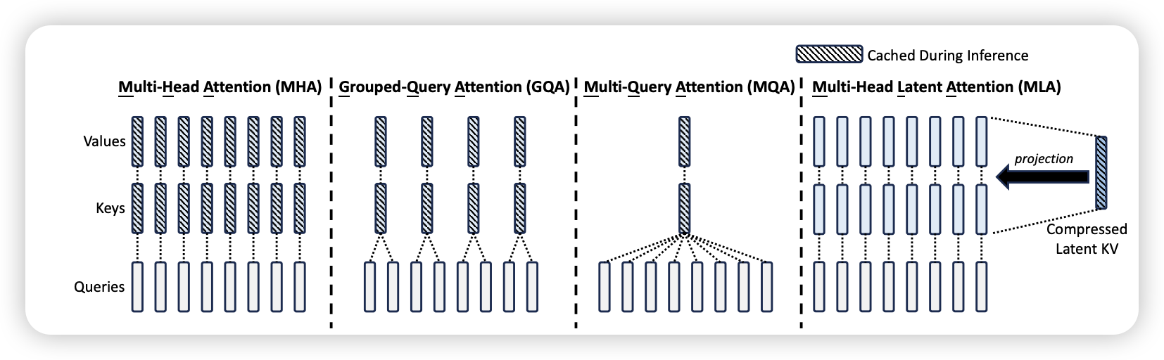
4.2 Grouped Query Attention / Multi Query Attention
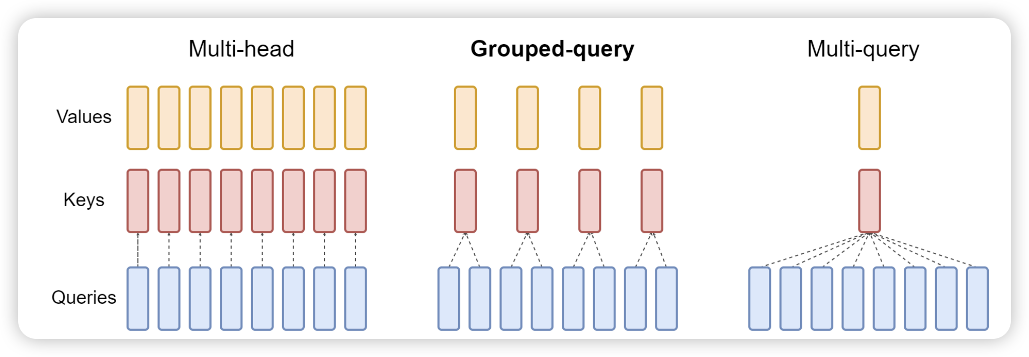
Proposed by the (Ainslie et al. 2023), Grouped Query Attention (GQA) and Multi Query Attention (MQA) are designed to reduce the computational burden of the attention mechanism by grouping queries and sharing keys and values across multiple queries.
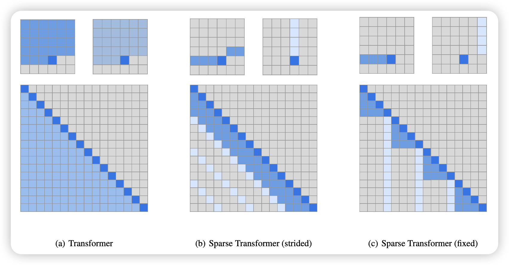
4.3 Sparse Attention
- Fixed Pattern Attention: for example, sliding window attention
- Strided Attention: for example, dilated attention, every m-th token
- Block Sparse Attention: for example, BigBird (BigBirdSparseAttention2020zaheer?), Longformer (Beltagy, Peters, and Cohan 2020)
- Global Attention:
- Learned / Dynamic Spare Attention
4.3.1 Sliding window attention
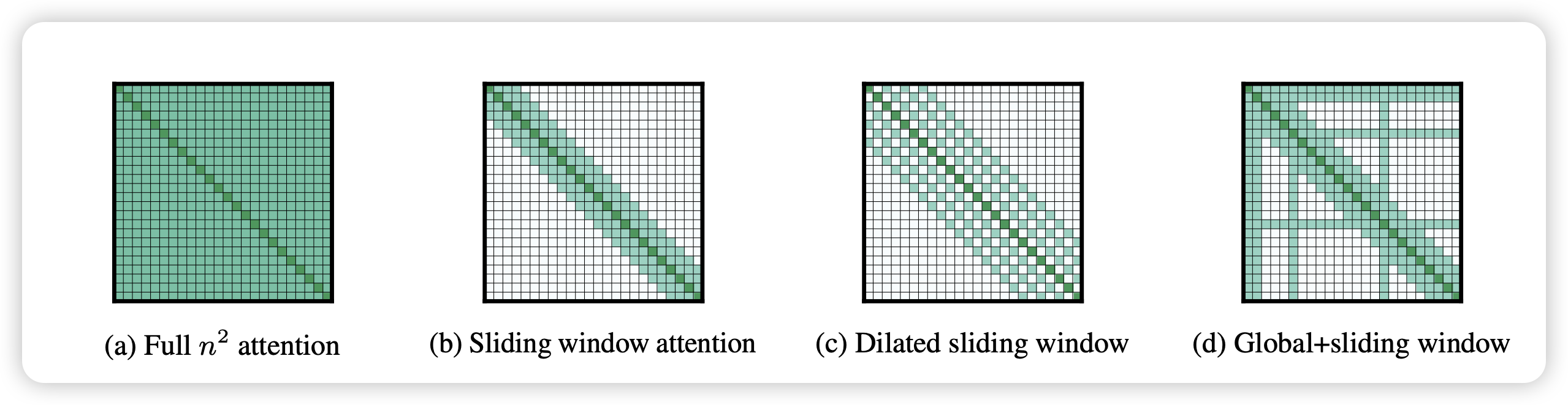
4.3.2 Dilated Attention
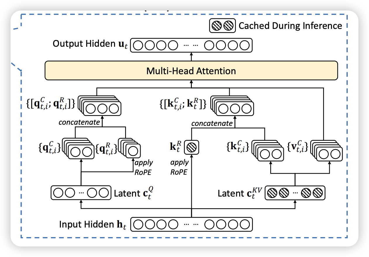
4.4 Multi Latent Attention
Multi Latent Attention (MLA), proposed in (DeepSeek-AI et al. 2024) is a proposed extension to the attention mechanism that aims to capture more complex relationships within the input data by introducing multiple latent spaces. Each latent space can learn different aspects of the data, allowing for a more nuanced understanding of the input.
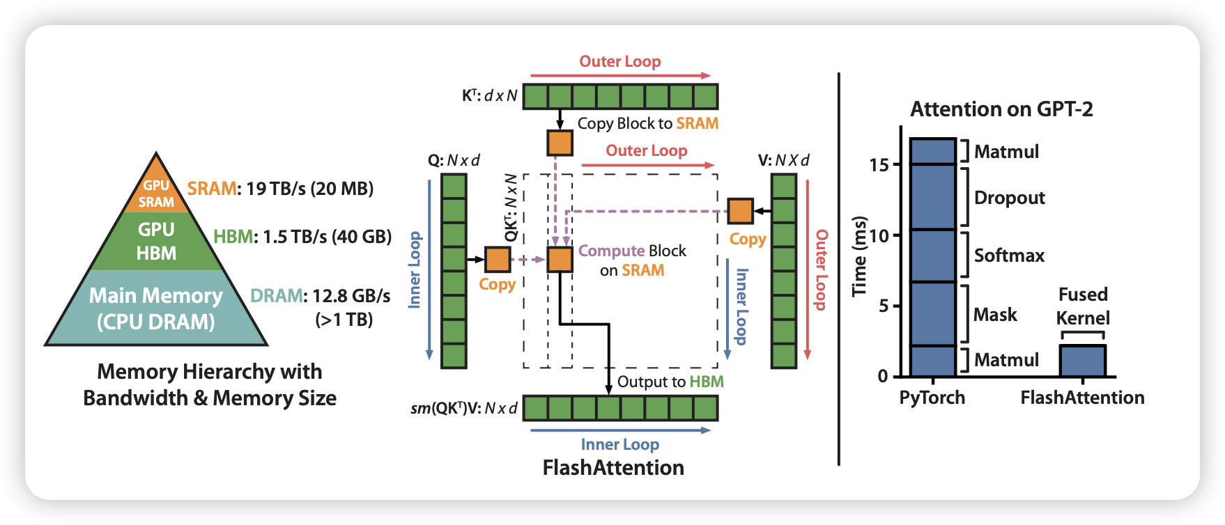
4.5 Flash Attention
So far, we see different attention mechanisms that aim to improve the efficiency and effectiveness of the standard attention mechanism. However, all aforementioned methods improve the attention mechanism by approximating the attention calculation. On the other hand, Flash Attention, proposed in (Dao 2023), takes a different approach by optimizing the attention computation itself.
4.5.1 Flash Attention V1 vs. V2 vs. V3
4.6 Native Sparse Attention
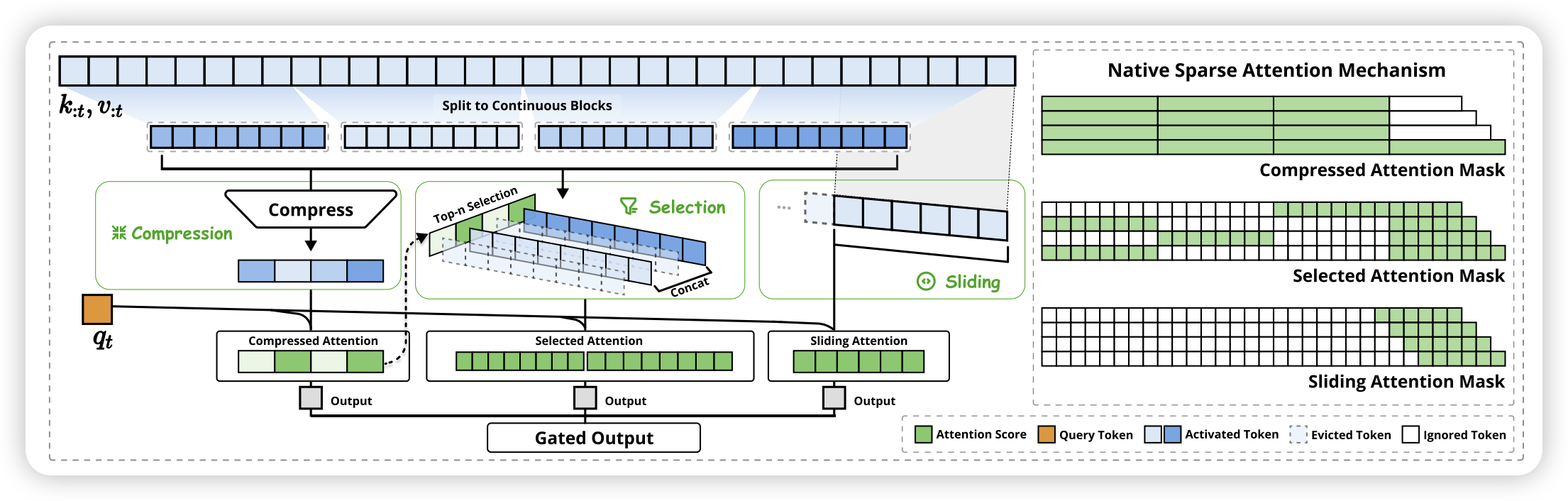
Proposed in (Yuan et al. 2025), this is a novel approach to sparse attention that aligns with hardware capabilities and allows for efficient training of sparse attention mechanisms.
4.7 Attention Sink
5 Activations
5.1 Swish
5.2 Gated Linear Unit (GLU)
6 Feed Forward Network & Mixture of Experts
6.1 Multi Layer Perceptron (MLP)
6.2 Gated Linear Unit (GLU)
6.3 Mixture of Experts (MoE)
7 Model Initialization
7.1 Weight Initialization
7.2 Layer Initialization
8 Case Study
Finally, we will examine some state-of-the-art LLM architectures and how they implement the techniques discussed in this blog.
8.1 LLaMA
8.2 Qwen
8.3 DeepSeek
8.4 GPT-Oss
9 Other Architectures
Right now, we just see all above model are transformer based architecture. But are they are the best solution? In the following, we will explore some alternative architectures that have been proposed.
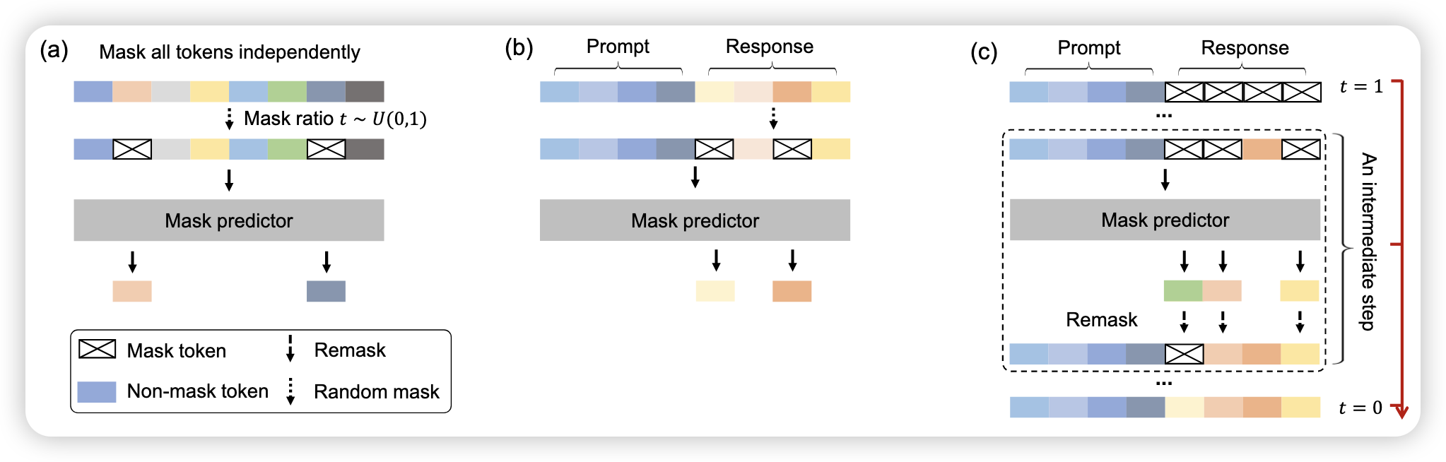
9.1 Diffusion Language Models
LLaDA (Nie et al. 2025) is a diffusion-based language model that leverages the principles of diffusion models to generate text. By modeling the text generation process as a diffusion process, LLaDA aims to improve the quality and diversity of generated text.

9.2 State Space Model (SSM)
10 Conclusion
This is conclusion