Stanford CS336: Language Modeling from Scratch
Lecture Website: Link
Lecture Video: YouTube
This is a collection of notes and code for the Stanford CS336: Language Modeling from Scratch course. This is course is designed to teach students how to build a “large” language model (LLM) from scratch, covering from bottom to top, including the:
- data collection and preprocessing,
- tokenization,
- model architecture and variations,
- pre-training,
- post-training,
- inference
- model evaluation.
The course is designed to provide a comprehensive understanding of how LLMs work and how to build them from scratch.
There are total
It might takes
Lectures
Lecture 01: Overview & Tokenization
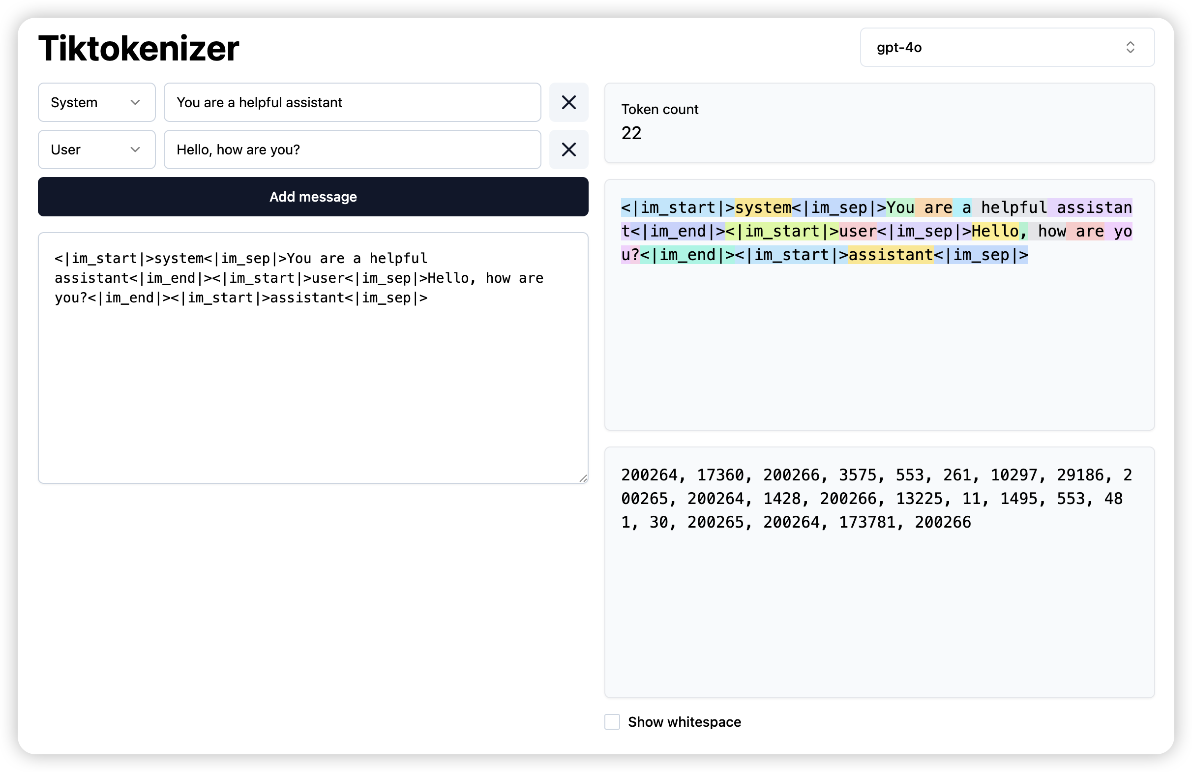
Byte Pair Encoding (BPE) is a simple yet effective tokenization algorithm that adaptively merges frequent character pairs to create a compact vocabulary, balancing compression efficiency and reversibility for language modeling.
Tokenization
Tokenization is the process of converting raw text into a sequence of tokens(usually is represented by integer indices), which are the basic units of meaning in a language model.
There are different level of tokenization, such as:
- Character-level: Each character is treated as a separate token.
- Word-level: Each word is treated as a separate token.
- Subword-level: Words are split into smaller units, such as prefixes, suffixes, or common subwords, to handle rare or out-of-vocabulary words more effectively.
- Byte-level: Each byte of the text is treated as a separate token, which can handle any character in the Unicode standard.
Before diving into the details of each tokenization algorithms , let’s first define a framework for tokenization in Python code: A Tokenizer is a class that implements the encode and decode methods for tokenization:
encode(string)method takes a string of text and converts it into a sequence of integer indices, which are the tokens.decode(indices)method takes a sequence of integer indices and converts it back into a string of text.
class Tokenizer:
    def __init__(self, config):

    def encode(self, string: str) -> list[int]:
        pass

    def decode(self, indices: list[int]) -> str:
        pass
The Tokenizer will generate a list of tokens from the input text, the number of the tokens is called the vocabulary size.
One of the good quantity to measure the tokenization algorithm is the compression ratio, which is defined as the ratio of the number of bytes of the input text to the number of tokens. A higher compression ratio indicates that the tokenization algorithm is more efficient in representing the input text. The compression ratio can be calculated as:
def get_compression_ratio(string: str, indices: list[int]) -> float:
    # Calculate the compression ratio of the tokenization algorithm
    return len(bytes(string, 'utf-8')) / len(indices)
Now, let’s discuss those four tokenization algorithms in detail:
Character-Based Tokenization
A Unicode string is a sequence of Unicode code points, which can be represented as a sequence of integers. Each character in the string is treated as a separate token, for example:
We can implement a simple character-based tokenizer as follows:
One of the main drawbacks of character-based tokenization is that it can lead to a large vocabulary size (there are approximately 150K unicode characters), which can make the model more difficult to train and less efficient in terms of memory usage. And some character are not commonly used in the text(e.g. ‘🌍’), which is inefficient use of the vocabulary.
Byte-Based Tokenization
Unicode strings can be encoded as a sequence of bytes using UTF-8 encoding. Each byte can be represented by integers in the range of 0 to 255. Some Unicode characters are represented by one byte, others take multiple bytes:
We can implement a simple byte-based tokenizer as follows:
As we can expected, the compression ratio is 1, which is terrible.
The vocabulary size is 256, which is a nice property because it is fixed and covers all possible bytes, which means we will not get out-of-vocabulary (OOV) tokens. However, the main drawback is that it can lead to long sequences, since each character (even multi-byte Unicode characters) is split into multiple tokens. This can make training less efficient and increase the computational cost for language models, given that the context length of a Transformer model is limited.
Word-Based Tokenization
Another common approach is to tokenize the text into words, where each word is treated as a separate token. We can use regular expression to split the text into words.
for example the GPT-2 regular expression is :
GPT2_TOKENIZER_REGEX = r"""'(?:[sdmt]|ll|ve|re)| ?\p{L}+| ?\p{N}+| ?[^\s\p{L}\p{N}]+|\s+(?!\S)|\s+"""
segments = re.findall(GPT2_TOKENIZER_REGEX, string)
After we get the segments, we can assign each segment to a unique integer index, which is the token. However there are several problem with this word-level tokenization:
- The number of words is huge.
- Many words are rare and the model won’t learn much about them.
- The vocabulary size is not fixed, which can lead to out-of-vocabulary (OOV) tokens. New words we haven’t seen during training will be treated as
UNKtokens, which can lead to a loss of information and context.
Byte Pair Encoding (BPE)
The basic idea of BPE is to iteratively merge the most frequent pairs of characters or subwords in the text until a desired vocabulary size is reached. This allows for a more efficient representation of the text, as it can capture common subwords and reduce the overall vocabulary size. The intuition behind BPE is that common sequences of characters are represented by a single token, rare sequences are represented by many tokens.
The GPT-2 paper used word-based tokenization to break up the text into initial segments and run the original BPE algorithm on each segment.
Here are the steps to implement BPE:
- Initialize: Start with a vocabulary that contains all unique characters in the text, usually start with 0-255
- Count Pairs: Count all adjacent character pairs in the text.
- Merge: Find the most frequent pair and merge it into a new token.
- Update: Replace all occurrences of the merged pair in the text with the new token.
- Repeat: Repeat steps 2-4 until the desired vocabulary size is reached.
@dataclass(frozen=True)
class BPETokenizerParams:
    vocab: dict[int, bytes]   # Mapping of token indices to byte sequences
    merges: dict[tuple[int, int], int]  # Mapping of pairs to their frequency

def merge(indices: list[int], pair: tuple[int, int], new_index:int)  -> list[int]:
    new_indices = []
    i = 0
    while i< len(indices):
        if i + 1 < len(indices) and indices[i] == pair[0] and indices[i + 1] == pair[1]:
            new_indices.append(new_index)  # Replace the pair with the new index
            i += 2  # Skip the next index since it's part of the pair
        else:
            new_indices.append(indices[i])  # Keep the current index
            i += 1  # Move to the next index
    return new_indices

class BPETokenizer(Tokenizer):
    def __init__(self, params: BPETokenizerParams):
        self.params = params

    def encode(self, string: str) -> list[int]:
        indices = list(map(int, string.encode('utf-8'))) # Convert string to byte indices
        for pair, new_index in self.params.merges.items():
            indices = merge(indices, pair, new_index)
        return indices

    def decode(self, indices: list[int]) -> str:
        byte_list = list(map(self.params.vocab.get, indices))  # Convert indices to bytes
        string = b''.join(byte_list)  # Join bytes into a single byte string
        return string.decode('utf-8')  # Decode byte string to UTF-8
To train an BPE tokenizer, we need to count the frequency of pairs in the text and merge them iteratively. The BPETokenizerParams class holds the vocabulary and merge rules, which can be generated from a training corpus.
def train_bpe_tokenizer(string: str, num_merges: int) -> BPETokenizerParams:
    # Initialize vocabulary with single characters
    vocab: dict[int, bytes] = {x: bytes([x]) for x in range(256)}  # index -> bytes, 256 unique bytes for UTF-8
    merges: dict[tuple[int, int], int] = {}  # index1, index2 => merged index

    # Convert string to byte indices
    indices = list(map(int, string.encode('utf-8')))

    for i in range(num_merges):
        # Count pairs
        counts = defaultdict(int)
        for index1, index2 in zip(indices[:-1], indices[1:]):
            counts[(index1, index2)] += 1

        # Find the most frequent pair

        most_frequent_pair = max(counts, key=counts.get)

        # Create a new token for the merged pair
        new_index = 256 + i
        merges[most_frequent_pair] = new_index
        vocab[new_index] = vocab[index1] + vocab[index2]  # Merge the byte sequences

        # Merge the pair in the indices
        indices = merge(indices, most_frequent_pair, new_index)

    return BPETokenizerParams(vocab=vocab, merges=merges)
We can save the BPETokenizerParams to a file and load it later to use the tokenizer. The BPE algorithm is efficient in terms of compression ratio, as it can adaptively merge frequent subwords to form a compact vocabulary, while still being reversible.
This implementation of BPE is a simplified version, and there are many optimizations and variations that can be applied to improve the efficiency and performance of the algorithm. For example, we can use a priority queue to efficiently find the most frequent pair. And we can also use more advanced techniques to speed up the merging process, such as caching and batching.
For those are more interested in the BPE, I highly recommend this video by Andrej Karpathy, which provides a detailed explanation of the BPE algorithm.
Summary of Lecture 01
In this lecture, we learned about the concept of the tokenization, which is the process of converting raw text into a sequence of tokens. We discussed four different tokenization algorithms: character-based, byte-based, word-based, and byte pair encoding (BPE). Each algorithm has its own advantages and disadvantages. We also learned how to measure the efficiency of a tokenization algorithm using the compression ratio. We will implemented more fancy version of the BPE algorithm in the assignment 01, which will be used to build a transformer model from scratch.
Below are the summary of four different tokenization algorithms:
| Tokenization Type | Description | Compression Ratio | Vocabulary Size | Pros | Cons |
|---|---|---|---|---|---|
| Character-Based | Each character is a token (Unicode code point). | Low | Large (all characters) | Simple; handles any language | Inefficient; large vocab; rare chars waste tokens |
| Byte-Based | Each byte from UTF-8 encoding is a token (0–255). | ~1 | Fixed (256) | Fixed vocab; language-agnostic | Long sequences for Unicode; inefficient for modeling semantics |
| Word-Based | Words (or regex-matched units) are tokens. | Medium | Large and dynamic | Intuitive; better compression than char/byte | Poor generalization; large vocab; OOV issues with UNK |
| Byte Pair Encoding (BPE) | Iteratively merges frequent subword pairs to form subword tokens. | High | Medium (tunable) | Efficient; balances granularity and vocab size | Merge rules are corpus-dependent; needs initial segmentation |
Lecture 02: Pytorch, Resource Accounting
h100_bytes = 80e9
Bytes_per_parameter = 4 + 4 + ( 4+ 4) => Parameters, gradient, optimizer state
Num Paramter = (h100_byes * 8) / Bytes_per_parameter 4e10
Memory Accounting
Let’s introduce three most common data types used in deep learning: float32, float16, and bfloat16.
float32 is the most common(default) data type used in deep learning, which uses 4 bytes per element.
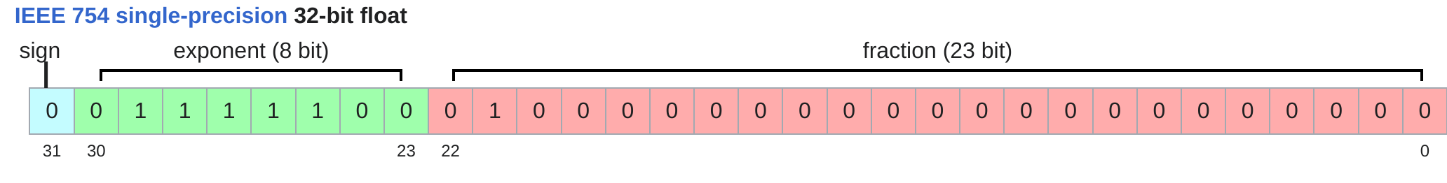
The exponent used to represent the dynamic range of the number, for float32, it uses 8 bits for the exponent, which allows for a dynamic range of approximately 1.18e-38 to 3.4e+38. The fraction is used to represent the precision of the number, which is also known as resolution. For float32, it uses 23 bits for the fraction, which allows for a precision of approximately 7 decimal digits. To represent a number in float32, it uses the following formula: \[
\begin{aligned}
\text{value}
&= (-1)^{b_{31}} \times 2^{(b_{30}b_{29} \dots b_{23})_2 - 127} \times (1.b_{22}b_{21} \dots b_{0})_2 \\
&= (-1)^{\text{sign}} \times 2^{(E - 127)} \times \left( 1 + \sum_{i=1}^{23} b_{23 - i} \cdot 2^{-i} \right)
\end{aligned}
\] where sign is the sign bit, exponent is the exponent value, and fraction is the fraction value. The exponent is biased by 127, which means that the exponent value is stored as the actual exponent plus 127. This allows for both positive and negative exponents to be represented.
Memory is determined by the number of values in the tensor and the data type of the tensor. The memory usage can be calculated as: \[ \text{Memory} = \text{Number of Values} \times \text{Bytes per Value} \tag{1}\] which can be calculated as:
The float32 takes 4 bytes per element, for the LLM, this is a lot of memory. We are use float16 to reduce the memory usage by half, which is 2 bytes per element. This is a common practice in deep learning to save memory and speed up training.
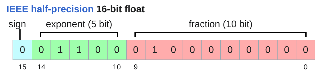
The float16 cuts down the memory usage by half, but it has a smaller dynamic range and precision compared to float32. This can lead to numerical instability and loss of precision in some cases, especially when dealing with very large or very small numbers.
when the underflow or overflow happens, the value will be rounded to 0 or infinity, which might cause the instability in the training process.
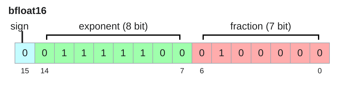
Another data type is bfloat16, which is a 16-bit floating point format that has the same dynamic range as float32, but with less precision. It uses 8 bits for the exponent and 7 bits for the fraction, which allows for a dynamic range of approximately 3.4e-38 to 3.4e+38, but with a precision of only 2 decimal digits.
In conclusion, the choice of data type can have a significant impact on the memory usage and performance of the model. The float32 is the most common data type used in deep learning, but it can be memory-intensive. The float16 and bfloat16 are commonly used to reduce the memory usage, but they can lead to numerical instability and loss of precision in some cases. One of the common practice to combine float16 and float32 is to use float16 for the model parameters and gradients, and float32 for the optimizer state. This is known as mixed precision training(Micikevicius et al. 2018), which can save memory and speed up training without sacrificing too much performance.
Compute Account
By defaults, all the tensors are stored in the CPU memory, which is not efficient for training deep learning models. We can move the tensors to the GPU memory by calling the to method on the tensor, which will move the tensor to the specified device.
x = torch.tensor([1, 2, 3])
x = x.to('cuda')  # Move tensor to GPU

num_gpus = torch.cuda.device_count() # Check the number of GPUs available
for i in range(num_gpus):
    properties = torch.cuda.get_device_properties(i)  # @inspect properties

y = x.to('cuda:0')  # Move tensor to GPU 0
One way to check the memory usage of the GPU in PyTorch is to use the torch.cuda.memory_allocated() and torch.cuda.memory_reserved() functions. The memory_allocated() function returns the total memory allocated by the tensors, while the memory_reserved() function returns the total memory reserved by the CUDA allocator.
The PyTorch tensor are pointers to the memory allocated on the GPU, with metadata such as the shape, data type, and device. There are several commom operations that can be performed on the tensors:
x = torch.tensor([[1., 2, 3], [4, 5, 6]])
y = x[0] # Get the first row of the tensor
z = x[:, 1] # Get the second column of the tensor
w = x[0, 1] # Get the element at the first row and second

y = x.view(3, 2) # Reshape the tensor to 3 rows and 2 columns
z = x.reshape(3, 2) # Reshape the tensor to 3 rows
w = x.transpose(0, 1) # Transpose the tensor
One of the most important operations in deep learning is the matrix multiplication, which can be performed using the torch.matmul() function. Also, besides that, the einops library provides a powerful way to manipulate tensors, allowing for more complex operations
Now, let’s talk about the compute account, which is the number of floating point operations (FLOPs) required to perform a certain operation. The FLOPs can be calculated as the number of floating point operations divided by the time taken to perform the operation.
The FLOPs is a measure of the computational complexity of an operation, and it is often used to compare the performance of different algorithms. The FLOP/s (FLOPs per second) is a measure of the performance of a hardware, which is the number of floating point operations that can be performed in one second. It is often used to compare the performance of different hardware, such as CPUs and GPUs.
Support we have a Linear layer with B batch size, D input dimension, and K output dimension. The number of floating point operations required to perform the forward pass of the linear layer can be calculated as:
where 2 is the number of floating point operations required to perform the matrix multiplication and addition (1 for multiplication and 1 for addition) of (i, j, k) triple.
Beside the matrix multiplication, the element-wise operations such as activation functions (e.g., ReLU, Sigmoid) also contribute to the FLOPs. For example, if we apply a ReLU activation function after the linear layer, it will add B * K additional floating point operations, since it applies the function to each element in the output tensor.
Addition of two \(m \times n\) matrices requires \(mn\) FLOPs, where \(m\) is the number of rows and \(n\) is the number of columns.
FLOPs is measure in terms of the number of the floating point operations required to perform a certain operation, which is a common way to measure the computational complexity of an algorithm. In theory, how to map those FLOPs to the wall clock time is not straightforward, since it depends on the hardware and the implementation of the algorithm. However, we can use the following formula to estimate the wall clock time:
One of the criterion is the MFU(Model FLOPs Utilization).Usually, MFU of >= 0.5 is quite good (and will be higher if matmuls dominate), the MFU is defined as the ratio of the number of floating point operations to the number of floating point operations that can be performed in one second, which is the FLOP/s. The MFU can be calculated as:
Eniops
It also introduce several einops operations:
einsumis used to perform Einstein summation notation, which is a powerful way to express complex tensor operations in a concise way.rearrangeis used to change the shape of the tensor without changing the data, it is similar tovieworreshapein PyTorch.reduceis used to reduce the tensor along a certain dimension, such as summing or averaging the values.repeatis used to repeat the tensor along a certain dimension, which is useful for broadcasting operations.
Count Flops for operations
A floating-point operation (FLOP) is a basic operation like addition (x + y) or multiplication (x y).
- FLOPs: floating-point operations (measure of computation done)
- FLOP/s: floating-point operations per second (also written as FLOPS), which is used to measure the speed of hardware.
For example, the Flops for the matrix multiplication of two matrices with dimensions m x n and n x p is 2 * m * n * p, where the 2 accounts for the multiplication and addition operations.
In the Linear module, the number of FLOPs can be calculated as follows:
Number of data points(B) x Number of parameters (D K)
One of the matrix is Model FLOPs utilization (MFU), which is the ratio of the number of floating point operations to the number of floating point operations that can be performed in one second, which is the FLOP/s. The MFU can be calculated as:
Models
Model Parameters Initialization
The model parameters are usually initialized using a random distribution, such as the normal distribution or the uniform distribution. Such as:
However, each element of output scales as sqrt(input_dim), so we need to scale the initialization by 1/sqrt(input_dim) to ensure that the variance of the output is not too large or too small. This is known as the Xavier initialization or Glorot initialization. The Xavier initialization can be implemented as follows:
To be more safe, we can truncate the normal distribution to avoid the outliers, which can be done by using the torch.nn.init.trunc_normal_ function. The truncation can be done by specifying the mean, std, and a and b parameters, which are the lower and upper bounds of the truncation.
Random Seed
To ensure the reproducibility of the results, we need to set the random seed for the random number generator. In PyTorch, we can set the random seed using the torch.manual_seed() function, which will set the seed for all the random number generators in PyTorch.
Data Loading
In language modeling, data is a sequence of integer (tokens) indices, It is convenient to serialize them as numpy arrays, and load it back.
If we don’t want to load the entire data into memory, we can use the np.memmap function to create a memory-mapped array, which allows us to access the data on disk as if it were in memory. This is useful for large datasets that cannot fit into memory.
data = np.memmap("data.npy", dtype=np.int32, mode="r")
print(data[0:10])  # Access the first 10 elements of the data
We can load data using
def get_batch(
    data: np.array,
    batch_size: int,
    sequence_length: int,
    device: str = "cpu"
) -> torch.Tensor:
    start_indices = torch.randint(len(data) - sequence_length, (batch_size, )) # Randomly select start indices for each batch
    batch = torch.stack([torch.tensor(data[i:i + sequence_length]) for i in start_indices])  # Create a batch of sequences
By default, CPU tensors are in paged memory, we can explicitly pin the memory to avoid the page faults, which can be done by using the pin_memory() method on the tensor. This will ensure that the tensor is allocated in a contiguous block of memory, which can improve the performance of the data loading process.
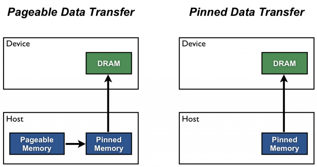
- Paged Memory: Default system memory that can be swapped out to disk by the OS. Slower transfer to GPU, and does not support asynchronous transfer.
- Pinned Memory: Also called page-locked or fixed memory. It is locked in RAM and cannot be swapped out. Enables faster transfer to GPU and supports asynchronous transfer.
This allows use to copy x from CPU to GPU asynchronously, which can improve the performance of the data loading process. We can use the to() method to move the tensor to the GPU, which will copy the tensor to the GPU memory.
This allows us to do two things in parallel (not done here):
- Fetch the next batch of data into CPU
- Process x on the GPU.
This is why when we load the data using the DataLoader in PyTorch, we can set the pin_memory=True to enable the pinned memory, which will automatically pin the memory for the tensors in the data loader. This can improve the performance of the data loading process, especially when using GPUs.
Optimizer
Introduce several common optimizers in PyTorch:
- SGD: Stochastic Gradient Descent, the most basic optimizer, which updates the parameters using the gradient of the loss function with a learning rate.
- Momentum: SGD + exponential averaging of gradients.
- Adaptive optimizers:
- Adam: Adaptive Moment Estimation, which uses the first and second moments of the gradients to adaptively adjust the learning rate for each parameter.
- Adagrad: Adaptive Gradient, which adapts the learning rate based on the historical gradients.
- RMSprop: Root Mean Square Propagation, which adapts the learning rate based on the historical squared gradients.
Implement of SGD optimizer in PyTorch is as follows:
class SGD(torch.optim.Optimizer):
    def __init__(self, params: Iterable[nn.Parameter], lr: float = 0.01):
        super(SGD, self).__init__(params, dict(lr=lr))
    def step(self):
        for group in self.param_groups:
            lr = group["lr"]
            for p in group["params"]:
                grad = p.grad.data
                p.data -= lr * grad
Also the AdaGrad optimizer can be implemented as follows:
class AdaGrad(torch.optim.Optimizer):
    def __init__(self, params: Iterable[nn.Parameter], lr: float = 0.01):
        super(AdaGrad, self).__init__(params, dict(lr=lr))
    def step(self):
        for group in self.param_groups:
            lr = group["lr"]
            for p in group["params"]:
                # Optimizer state
                state = self.state[p]
                grad = p.grad.data
                # Get squared gradients g2 = sum_{i<t} g_i^2
                g2 = state.get("g2", torch.zeros_like(grad))
                # Update optimizer state
                g2 += torch.square(grad)
                state["g2"] = g2
                # Update parameters
                p.data -= lr * grad / torch.sqrt(g2 + 1e-5)
The usage of the optimizer is as follows:
model = MyModel()
optimizer = torch.optim.SGD(model.parameters(), lr=0.01)

x_in = torch.randn(32, 100)  # Input tensor
y_out = model(x_in)  # Forward pass
target = torch.randn(32, 10)  # Target tensor
loss = loss_fn(y_out, target)  # Compute loss

loss.backward()  # Backward pass
optimizer.step()  # Update parameters
optimizer.zero_grad(set_to_none=True) # Zero gradients for the next iteration # Set to None is more memory efficient
Training Loop
Checkpointing
Mixed Precision Training
Choice of data type (float32, bfloat16, fp8) have tradeoffs.
Higher precision: more accurate/stable, more memory, more compute
Lower precision: less accurate/stable, less memory, less compute
We can use mixed precision training to balance the tradeoffs, which is a common practice in deep learning to save memory and speed up training without sacrificing too much performance. The idea is to use float16 bfloat16 for the model parameters and gradients, and float32 for the optimizer state. This can be done using the torch.cuda.amp module in PyTorch, which provides automatic mixed precision training.
scaler = torch.cuda.amp.GradScaler()  # Create a GradScaler for mixed precision training
for data, target in dataloader:
    optimizer.zero_grad(set_to_none=True)  # Zero gradients for the next iteration
    with torch.cuda.amp.autocast():  # Enable autocasting for mixed precision training
        output = model(data)  # Forward pass
        loss = loss_fn(output, target)  # Compute loss
    scaler.scale(loss).backward()  # Backward pass with scaled loss
    scaler.step(optimizer)  # Update parameters with scaled gradients
    scaler.update()  # Update the scaler for the next iteration
Summary of Lecture 02
Lecture 03: Architectures & Hyperparameters
Lecture 04: Mixture of Experts
Lecture 05 & 06: GPU, Kernels, Triton
Lecture 07 & 08: Parallelism
Lecture 09 & 11: Scaling Laws
Lecture 10: Inference
Lecture 12: Evaluation
Lecture 13 & 14: Data
Lecture 15, 16 & 17: Alignment: SFT/ RLHF
Assignments
Assignment 01: Basics
Preparation
Clone Assignment Repository
First, we need clone the assignment repository from GitHub:
git clone https://github.com/stanford-cs336/assignment1-basics/tree/main
cd assignment1-basics
Download Dataset
Then, we need download the dataset, the dataset used are TinyStories and OpenWebText
mkdir -p data
cd data

wget https://huggingface.co/datasets/roneneldan/TinyStories/resolve/main/TinyStoriesV2-GPT4-train.txt
wget https://huggingface.co/datasets/roneneldan/TinyStories/resolve/main/TinyStoriesV2-GPT4-valid.txt

wget https://huggingface.co/datasets/stanford-cs336/owt-sample/resolve/main/owt_train.txt.gz
gunzip owt_train.txt.gz
wget https://huggingface.co/datasets/stanford-cs336/owt-sample/resolve/main/owt_valid.txt.gz
gunzip owt_valid.txt.gz

cd ..
After downloading the dataset, we can check the size of the dataset:
du -sh ./data
# 13G    ./data
There are 13GB of data in total, which is a small dataset for training a language model.
Install Dependencies
To run code, and install the dependencies, we can just run the following command:
uv run pythonIt will automatically create a virtual environment and install the dependencies.
Byte-Pair Encoding (BPE) Tokenizer
The Unicode Standard
ord() # convert a single Unicode character into its integer representation
chr() # convert a single integer representation into its Unicode character
The Unicode character chr(0) return '\x00', which is the null character. While use repr(chr(0)) will return "'\\x00'", which is the string representation of the null character. When use print function, it will not print anything, since the null character is not printable. So, when add the chr(0) to the string, it will not change the string, but it will add a null character to string.
Unicode Encoding
Unicode Encoding is the process of converting a Unicode character into a sequence of bytes. The most common encoding is UTF-8, which uses 1 to 4 bytes to represent a Unicode character.
Unicode Standard is a character encoding standard that defines a unique number for every character, no matter the platform, program, or language. Unicode Encoding is the actual implementation of the Unicode Standard in a specific encoding format, such as UTF-8 or UTF-16. It will convert the Unicode character into a sequence of bytes.
To encode the Unicode string into UTF-8, we can use the encode() method in Python to convert the string into a byte sequence, and then use the decode() method to convert the byte sequence back into a string. The encode() method takes an optional argument that specifies the encoding format, which is UTF-8 by default.
original_string = "Hello World! 🌍 你好, 世界!"
utf8_encode = original_string.encode("utf-8")
utf8_bytes = list(utf8_encode) # Get the byte values of the encoded string
original_string = utf8_encode.decode("utf-8")
len(original_string) # 22
len(utf8_bytes) # 33
UTF-8 is variable-length and uses 1 byte for ASCII (common in English), making it more compact for most real-world text. UTF-16 uses 2 or 4 bytes per character, and UTF-32 always uses 4 bytes, even for ASCII.
s = "hello"
print(len(s.encode("utf-8")))   # 5 bytes
print(len(s.encode("utf-16")))  # 12 bytes (includes BOM)
print(len(s.encode("utf-32")))  # 20 bytes (includes BOM)
UTF-8 produces a byte range of 0–255, making the vocabulary size small and fixed (ideal for BPE training).
• UTF-16/32 would increase the vocabulary size dramatically (≥65,536 for UTF-16 and ~4 billion for UTF-32), requiring larger models and memory.bytes() creates an immutable sequence of bytes — that is, a sequence of integers in the range 0–255.
s = "hello 🌍"
b = bytes(s, "utf-8")
print(b)  # b'hello \xf0\x9f\x8c\x8d'
b = s.encode("utf-8")

b = bytes([104, 101, 108, 108, 111])  # equivalent to 'hello'
print(b)  # b'hello'

b = bytes(5)
print(b) # b'\x00\x00\x00\x00\x00'The function is incorrect because it decodes each byte individually, but multi-byte UTF-8 characters (like ‘🌍’) must be decoded as a whole sequence, not byte-by-byte.
BPE Tokenizer Training
Three steps:
- Vocabulary Initialization
- Pre-Tokenization
- Compute BPE merges
- Handle Special Tokens
Assignment 02: System
In this assignment, we will profile and benchmark the model we built in the assignment 01, and optimize the attention mechanism using Triton by implementing the FlashAttention2(Dao 2023).