Speed Up Training for Neural Networks

Training Tricks

Training large neural networks can be time-consuming and resource-intensive. This blog post explores various techniques to speed up the training process, including optimizing calculating in the single GPUs, and parallelizing the training across multiple GPUs.

Author

Yuyang Zhang

Published

2025-08-07

Last modified

2025-08-07

Training large neural networks(such as large language models) can be time-consuming and resource-intensive. This blog post explores various techniques to speed up the training process, including optimizing calculations on a single GPU through different techniques such as fusion, tiling, memory coalescing, and parallelizing the training across multiple GPUs such as model parallelism and data parallelism. But before that, we need to understand the basic concepts of GPU, and data types to better understand why and when we need to use these techniques.

1 Preliminary

1.1 Data Representation

In deep learning, we often use different data types to represent our data and model parameters. The most common data types are:

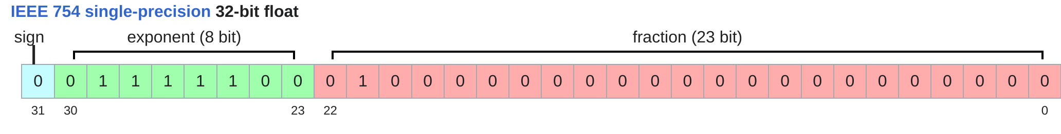
Float32: also known as single-precision floating-point format. This is the default floating-point representation used in most deep learning frameworks. It provides a good balance between precision and performance. It use 32 bits (4 bytes) to represent a number.
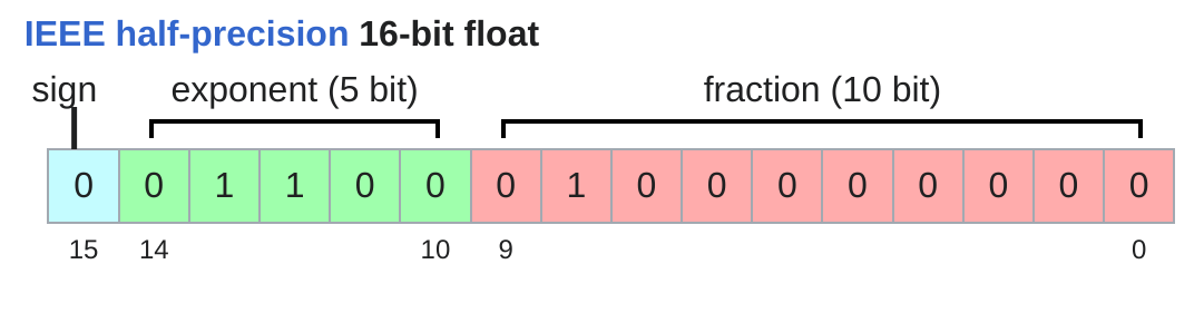
Float16: This is a half-precision floating-point representation that uses 16 bits instead of 32 bits. It can significantly speed up training and reduce memory usage, but it may lead to numerical instability in some cases.
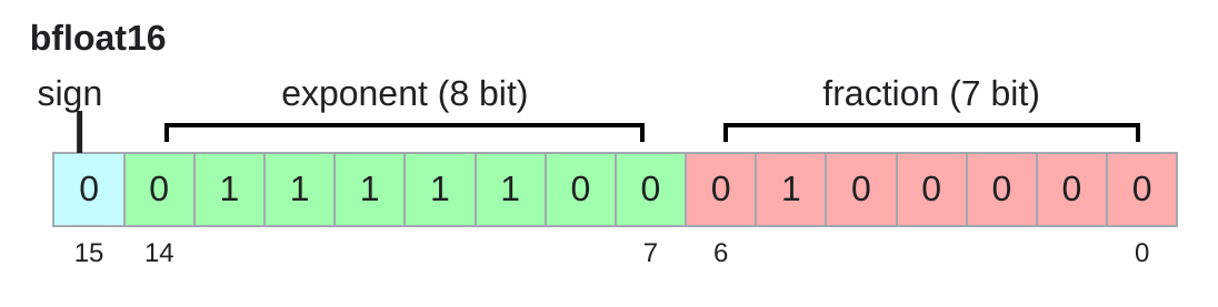
BFloat16: This is a truncated version of Float32 that retains the exponent bits but reduces the mantissa bits. It is designed to provide a good trade-off between precision and performance, especially for training large models.

How those bits represent the number?

\[ \text{value} = (-1)^s \times (1.f) \times 2^{e - 127} \]

where:

\(s\) is the sign bit (0 for positive, 1 for negative)
\(f\) is the mantissa (the fractional part): \(1.f = 1 + \sum_{i=1}^{23} b_i \cdot 2^{-i}\), where \(b_i\) are the bits of the mantissa either 0 or 1.
\(e\) is the exponent (an 8-bit unsigned int) with a bias of 127:
- For Float32, \(e\) is 8 bits, which range from [1, 254]
- For Float16, \(e\) is 5 bits, which range from [1, 30]
- For BFloat16, \(e\) is 8 bits, which range from [1, 254]

To check the data type of a tensor and its properties in PyTorch, you can use the .dtype attribute. For example:

x = torch.zeros(4, 8)
x.dtype # check the data type of x
x.numel() # check the number of elements in x
x.element_size() # check the size of each element in bytes
x.numel() * x.element_size() # check the total size in bytes

1.2 Calculate Memory Usage of Model

Assume we have a model with \(N\) parameters, and each parameter is represented by float32 (4 bytes). \(A\) is the number of activation elements stored during forward (depends on input and model depth). How can we calculate the memory need for training this model? Notice that the memory usage of a model is not only determined by the parameters, but also by:

activations
gradients
optimizer states

For a single parameter, the memory usage for one forward pass and backward pass is:

parameter: 4 bytes (float32)
activation: 4 bytes (float32)
gradient: 4 bytes (float32)
optimizer state, which can vary depending on the optimizer used. For example, Adam optimizer requires 2 additional states (momentum and variance), each of which is 4 bytes (float32).

So, the total memory usage for one parameter is: \[ \text{Memory per parameter} = 4 + 4 + 2 \times 4 = 16 \text{ bytes} \]
Thus, the total memory usage for the model is: \[ \text{Total Memory} = N \times 16 \text{ bytes} + A \times 4 \text{ bytes} \]

Why need activation for backward pass?

Say a layer denotes the input to the layer as \(\mathbf{x}\), the weights as \(\theta\), and the output as \(\mathbf{y}\). The loss function is denoted as \(L\), which is a function of the output \(\mathbf{y}\) and the target \(t\): \[ \mathbf{y} = f(\mathbf{x}; \theta) \] To compute the gradient of the loss with respect to the weights, we need to use the chain rule: \[ \frac{\partial L}{\partial \theta} = \frac{\partial L}{\partial \mathbf{y}} \cdot \frac{\partial \mathbf{y}}{\partial \theta} \]

where \(\frac{\partial \mathbf{y}}{\partial \theta}\) is the gradient of the output with respect to the weights \(\theta\), which usually are the function of the input \(\mathbf{x}\) and the weights \(\theta\). To compute this gradient, we need to know the input \(\mathbf{x}\). For example, the linear layer computes: \[ \mathbf{y} = \mathbf{x} \cdot \theta + b \] to compute the gradient, we need to know the input \(\mathbf{x}\), \[ \frac{\partial L}{\partial \theta} = \frac{\partial L}{\partial \mathbf{y}} \cdot \mathbf{x} \] where \(\mathbf{x}\) is the input to the layer, which is the activation of the previous layer. Thus, we need to store the activation for the backward pass.

Calculate Memory Usage of Model

import torch
import torch.nn as nn

# Set device
device = torch.device("cuda" if torch.cuda.is_available() else "cpu")

# Define a simple model
model = nn.Sequential(
    nn.Linear(100, 200),
    nn.ReLU(),
    nn.Linear(200, 50),
    nn.ReLU(),
    nn.Linear(50, 10)
).to(device)

# Register hooks to track activation sizes
activation_sizes = []

def hook_fn(module, input, output):
    if isinstance(output, torch.Tensor):
        activation_sizes.append(output.numel())
    elif isinstance(output, (list, tuple)):
        activation_sizes.extend(o.numel() for o in output if isinstance(o, torch.Tensor))

hooks = []
for layer in model:
    hooks.append(layer.register_forward_hook(hook_fn))

# Create input
x = torch.randn(32, 100, device=device, requires_grad=True)

# Forward pass
output = model(x)
loss = output.mean()

# Backward pass
loss.backward()

# Remove hooks
for h in hooks:
    h.remove()

# --------- Memory Estimation ---------
# 1. Parameters
num_params = sum(p.numel() for p in model.parameters())
param_memory = num_params * 4
grad_memory = num_params * 4
optimizer_memory = num_params * 8

# 2. Activations (sum of all layer outputs + input)
activation_memory = (x.numel() + sum(activation_sizes)) * 4  # float32

# 3. Total
total_bytes = param_memory + grad_memory + optimizer_memory + activation_memory
total_MB = total_bytes / (1024 ** 2)

# Print
print(f"Total parameters: {num_params}")
print(f"Activation elements: {sum(activation_sizes)}")
print(f"Total training memory (float32): {total_MB:.2f} MB")

1.3 Collective operations

Collective operations are operations that involve multiple processes or devices, such as GPUs, to perform a computation. They are essential for parallelizing the training process across multiple GPUs. Some common collective operations include:

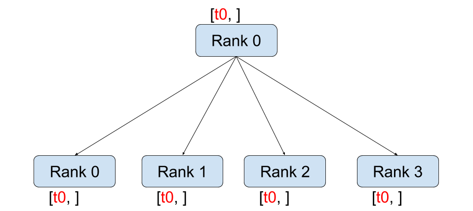
Broadcast(Figure 2 (a)): This operation sends data from one process to all other processes. It is commonly used to share model parameters or hyperparameters across multiple GPUs.
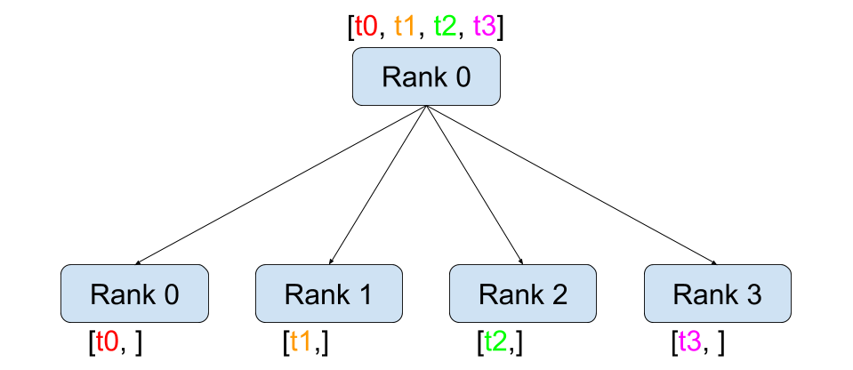
Scatter(Figure 2 (b)): This operation distributes data from one process to multiple processes. It is often used to distribute input data across multiple GPUs.
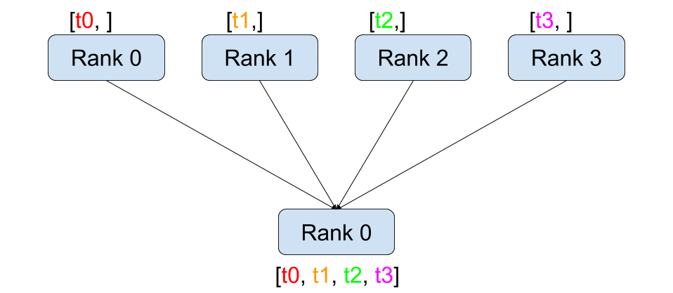
Gather(Figure 2 (c)): This operation collects data from multiple processes and combines it into a single process. It is useful for aggregating results from multiple GPUs.
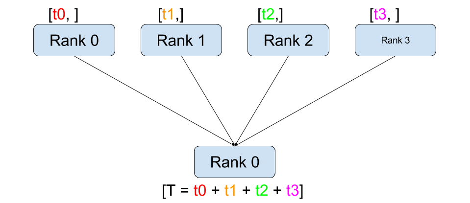
Reduce(Figure 2 (d)): This operation combines data from multiple processes into a single process. It is commonly used to compute the sum or maximum of gradients across multiple GPUs.
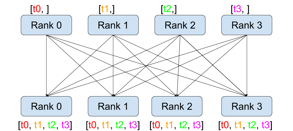
All-gather(Figure 2 (e)): This operation collects data from all processes and distributes it back to all processes. It is often used to gather gradients or model parameters from multiple GPUs without losing any information.
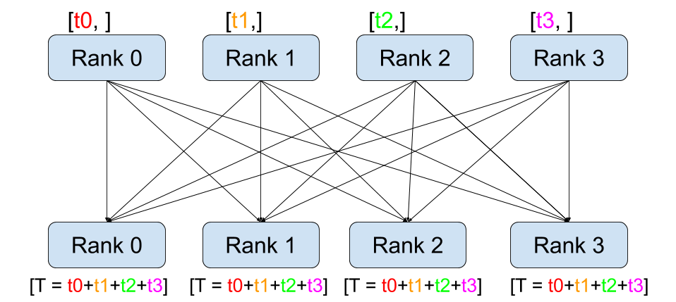
All-reduce(Figure 2 (g)): This operation combines data from all processes and distributes the result back to all processes. It is often used to average gradients across multiple GPUs during training.
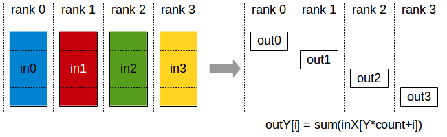
Reduce-scatter(Figure 2 (f)): This operation combines data from multiple processes and distributes the result to each process. It is often used to reduce the amount of data that needs to be communicated between processes.

One should take note is Reduce-Scatter combines two operations:

Reduce: Each process (or GPU) contributes its data, and a reduction operation (usually sum, mean, max, etc.) is applied across processes.
Scatter: The reduced result is partitioned and each process gets only a portion (its shard) of the reduced result.

Tip

Way to remember the terminology:

Gather: collects data from multiple sources into one destination(not do any operation)
Reduce: performs some associative/commutative operation (sum, min, max)
Broadcast/Scatter: is inverse of Gather
All: means destination is all devices

2 Profiling

To optimize the training process, we need to first profile our model to identify the bottlenecks. In this section, we will introduce several tools to profile the model and understand where the time is spent during training. We will discuss several tools that can help us profile our model and identify the bottlenecks in the training process:

Simple Benchmarking (Section 2.1): The simplest way to measure the time taken for each operation in your model. You can use the time module in Python to measure the time taken for each operation. For example, you can wrap your forward pass in a timer to measure the time taken for each layer.
PyTorch Profiler (Section 2.2): PyTorch provides a built-in profiler that can help you analyze the performance of your model. You can use the torch.profiler module to profile your model and visualize the results. The profiler provides detailed information about the time spent on each operation, memory usage, and more.
NVIDIA Nsight Systems (Section 2.3): This is a powerful profiling tool that can help you analyze the performance of your model on NVIDIA GPUs. It provides detailed information about the GPU utilization, memory usage, and more. You can use it to identify bottlenecks in your model and optimize the performance.

2.1 Simple Benchmarking

2.2 PyTorch Profiler

2.3 NVIDIA Nsight Systems

3 Single GPU Optimization

In this section, we will discuss various techniques to optimize the training process on a single GPU. These techniques include: - Fusion(Section 3.1): This technique combines multiple operations into a single operation to reduce the number of kernel launches and improve performance. For example, you can fuse the forward and backward passes of a layer into a single operation. - Tiling(Section 3.2): This technique divides the input data into smaller tiles and processes them in parallel to improve memory access patterns and reduce memory usage. For example, you can tile the input data into smaller chunks and process them in parallel. - Memory Coalescing(Section 3.3): This technique optimizes memory access patterns to improve memory bandwidth utilization. For example, you can coalesce memory accesses to reduce the number of memory transactions and improve performance. - Mixed Precision Training(Section 3.4): This technique uses lower precision data types (such as float16 or bfloat16) to reduce memory usage and improve performance. It can significantly speed up training while maintaining model accuracy. PyTorch provides built-in support for mixed precision training through the torch.cuda.amp module, which allows you to automatically cast your model and inputs to lower precision during training. - Gradient Accumulation(Section 3.5): This technique accumulates gradients over multiple mini-batches before performing a weight update. It can help reduce the number of weight updates and improve training stability, especially when using large batch sizes. You can implement gradient accumulation by accumulating gradients in a buffer and updating the model parameters only after a certain number of mini-batches.

3.1 Fusion

3.2 Tiling

3.3 Memory Coalescing

3.4 Mixed Precision Training

3.5 Gradient Accumulation

3.6 Case Study: Flash Attention

4 Multi-GPU Optimization(Parallelism)

In this section, we will discuss various techniques to optimize the training process across multiple GPUs. These techniques include: - Data Parallelism(Section 4.1): This technique splits the input data across multiple GPUs and performs the forward and backward passes in parallel. Each GPU processes a different subset of the input data, and the gradients are averaged across GPUs before updating the model parameters. - Model Parallelism(Section 4.2): This technique splits the model across multiple GPUs and performs the forward and backward passes in parallel. Each GPU processes a different part of the model, and the gradients are averaged across GPUs before updating the model parameters. This is particularly useful for large models that do not fit into a single GPU’s memory. - Pipeline Parallelism(Section 4.3): This technique splits the model into multiple stages and processes each stage in parallel across multiple GPUs. Each GPU processes a different stage of the model, and the output of one stage is passed to the next stage. This can help improve throughput and reduce memory usage, especially for large models. - Tensor Parallelism(Section 4.4): This technique splits the tensors across multiple GPUs and performs the forward and backward passes in parallel. Each GPU processes a different part of the tensor, and the gradients are averaged across GPUs before updating the model parameters. This is particularly useful for large tensors that do not fit into a single GPU’s memory. - Context Parallelism(Section 4.5): This technique splits the context across multiple GPUs and performs the forward and backward passes in parallel. Each GPU processes a different part of the context, and the gradients are averaged across GPUs before updating the model parameters. This is particularly useful for large contexts that do not fit into a single GPU’s memory.

4.1 Data Parallelism

4.2 Model Parallelism

4.3 Pipeline Parallelism

4.4 Tensor Parallelism

4.5 Context Parallelism

4.6 Case Study: DeepSpeed

4.7 Case Study: Megatron-LM

Name	Self CPU %	Self CPU	CPU total %	CPU total	CPU time avg	Self CUDA	Self CUDA %	CUDA total	CUDA time avg	# of Calls
aten::gelu	6.76%	669.785us	13.48%	1.336ms	1.336ms	8.642ms	100.00%	8.642ms	8.642ms	1
void at::native::vectorized_elementwise_kernel<…>	0.00%	0.000us	0.00%	0.000us	0.000us	8.642ms	100.00%	8.642ms	8.642ms	1
cudaLaunchKernel	6.72%	665.807us	6.72%	665.807us	665.807us	0.000us	0.00%	0.000us	0.000us	1
cudaDeviceSynchronize	86.52%	8.574ms	86.52%	8.574ms	4.287ms	0.000us	0.00%	0.000us	0.000us	2

Self CPU time total: 9.909 ms
Self CUDA time total: 8.642 ms